Recently, the issue of the limited supply of radio spectrum resources has become a growing concern due to the enormous demand for wireless communication services. At the same time, the current system of fixed allocation of the spectrum leads to low usage for most of the spectrum, according to the research of the US Federal Communi-cations Commission (FCC) [1]. In the face of this so-called “spectral crisis”, Mitola [2] proposed the concept of ‘cognitive radio (CR)’.

Wireless communication technology has entered the era of 4G/5G. The demands for higher data transmission speed through wireless communication systems increase with each passing day. How to improve the reliability and bandwidth efficiency of the system has become the vital target of wireless communication technology design in the next generation and beyond. Transmitting data streams using multiple antennas, known as multiple-input/multiple-output (MIMO), can increase the capacity and bandwidth efficiency of communication systems significantly without greatly increasing the system bandwidth at the same time. This is considered one of the key technologies of modern wireless communication [1]. However, MIMO has some drawbacks [2]: high inter-antenna synchronization is required among transmitting antennas to meet the demand of simultaneous data transmissions; simultaneous data transmissions by multiple antennas can cause high inter-channel interference (ICI), which increases the difficulty of decoding, as well as the complexity of the system; and multiple RF chains are needed when multiple antennas work at the same time, increasing system costs.

A CR system is an intelligent radio communication system that is able to sense the surrounding radio envi-ronment and analyze the sensed result. Then the radio operating parameters will be dynamically adjusted in real time on the basis of that result [3]. The drawbacks of the present spectrum allocation scheme can be resolved effect-tively by the secondary utilization of spectrum resources. According to the IEEE 802.22.1 standard [4], the secondary user (SU) should detect TV and broadcast signal and idle channels within 2 seconds, which requires cognitive users to access and exit the frequency band authorized by the primary user (PU) promptly, on the premise of guaranteed high detection probability.

The existing spectrum sensing algorithms can be roughly classified into three categories:

On account of the problems with the existing algorithms, the concept of using the generalized likelihood ratio has been raised [9]. In a multi-antenna system, when there is only one PU in the space, the structural properties of the received signal can be utilized to design an algorithm. In such a case, the application environment is more realistic because only a small number of sample points are involved. This algorithm has a higher detection performance under a low signal-to-noise ratio (SNR). However, this algorithm is only appropriate for a situation with one PU, while real situations usually involve several PUs at the same time. The detection performance of this algorithm can drop off severely when several PUs exist.

So far, most eigenvalue-based spectrum sensing algo-rithms have been designed based on the analysis of detection performance using random matrix theory (RMT) [10], and significant branches of RMT can be classified into asymptotic theory and non-asymptotic theory. Asymptotic theory studies the convergence property of the spectrum distribution function of the random matrix in infinite dimensional space. These concepts have now been quite thoroughly explored, and asymptotic theory has already been widely applied to all kinds of proposed eigenvalue algorithms. Meanwhile, non-asymptotic theory [11] is the latest achievement within RMT: the convergence property of the spectrum distribution function of the random matrix in finite-dimensional space. In an actual situation, the number of sampling points is usually small; thus non-asymptotic theory is more widely applicable.

Meanwhile, existing eigenvalue algorithms only use the characteristics of some particular eigenvalues, for example, the maximum eigenvalue, the minimum eigenvalue, and the ratio of the maximum and minimum eigenvalue. Other eigenvalues have not been used. Therefore, the purpose of this paper is to excavate potential uses of these neglected eigenvalues and design eigenvalue detection algorithms with joint distribution of eigenvalues, in order to improve the performance of spectrum sensing.

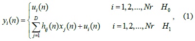
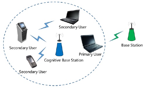
A typical multi-antenna spectrum sensing scenario is as shown in Fig. 1. In the space, the number of PUs is D and the number of SUs is K. The multi-antenna system is applied to the SUs, the receiving equipment has Nr receiving antennas, and each antenna has N sampling signals. There are two hypotheses on whether a PU’s signal exists. H₀ represents the situation in which the PU does not exist, and there is only noise, while H₁ represents the situation in which both the PU and noise exist. The spectrum sensing model of a multi-antenna CR system can be described as a binary hypothesis model:

where i=1,2,3…Nr denotes i receiving antennas of the SU; y_i(n) denotes the signal received from the PU at receiving antenna i; x_i(n) is the transmitting signal of the j^th PU; h_ij(n) is the channel gain between the ith receiving antenna and the j^th PU; and u_i(n) is the Gaussian white noise with its mean value as 0 and variance as .

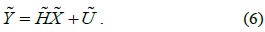
The statistical matrix of the received signal at the SU can be expressed as follows:

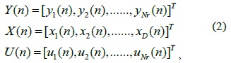
where y_i(n) , x_i(n) , and u_i(n) are an N×1 vector. According to the definition of matrix, (1) can be expressed as

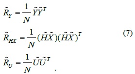
The covariance matrix of the received signal is thus

From (3) and (4),

In an actual algorithm, to approximate an observed signal with finite sampling points N, (2) can be written in the form of an Nr×N estimate covariance matrix:

With (4) recalculated,

Suppose that the eigenvalues of the sampling covariance matrix are λ₁=λ_max≥λ₂≥…≥λ_Nr=λ_min , and the eigenvalues of the covariance matrix are ρ₁=ρ_max≥ρ₂…≥ρ_Nr=ρ_min . From Eq. (7), If there is no PU signal, ρ_max=ρ_min=0 and thus

Based on the analysis of the system model, we can use eigenvalues of the received signal to detect whether there is a PU. For the detection threshold γ of the detection algorithm, if the detection statistic T<γ, a PU does not exist, indicating that H₀ is confirmed; if T>γ , a PU exists, confirming H₁.

Many spectrum-sensing algorithms have been developed based on eigenvalues. Relatively speaking, the maximum-minimum eigenvalue (MME) algorithm based on RMT is a classic one. In light of the drawbacks of its performance, taking the pre-difference, Lagrange’s interpolation, and the double threshold method, for example, is put forward. What is undeniable is that most of the algorithms have only used the properties of some eigenvalues. The algorithms proposed in this paper were developed with the goal of finding effective detection algorithms that use the joint distribution properties of the received signal’s eigenvalues. The existing algorithms and proposed algorithms can be classified as follows.

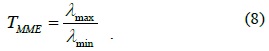
1) Maximum-Minimum Eigenvalue

When H₀ is true, the ratio of the maximum and minimum eigenvalues is 1, and when H₁ is true, the ratio of the maximum and minimum eigenvalues is According to the difference of the ratios under the two hypotheses, the MME algorithm uses λ_max / λ_min as the test statistic to decide whether the PU exists or not.

If T_MME>γ_MME , then there are PUs in the space. On the other hand, if T_MME<γ_MME , then the space contains no PUs. γ_MME represents the detection threshold of the MME algorithm.

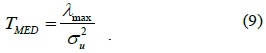
2) Maximum Eigenvalue Detection

Under a binary hypothesis, H₀ indicates a lack of PUs, and thus while H₁ indicates the presence of a PU and Therefore, the ratio of the maximum eigenvalue and noise variance under the two hypotheses can be used as the detection statistic, written as follows:

If T_MAX>γ_MAX , then there are PUs in the space, and vice versa. γ_MAX represents the detection threshold of the maximum eigenvalue detection (MED) algorithm.

3) Generalized Likelihood Ratio Test

Under a binary hypothesis regarding the CR system, the general model of the generalized likelihood ratio can be written as follows:

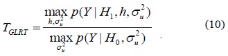
In accordance with the maximum likelihood estimation, the detection statistic can be determined by

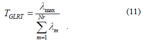
If T_GLRT>γ_GLRT , then there are PUs in the space, and vice versa. γ_GLRT represents the detection threshold of the generalized likelihood ratio test (GLRT) algorithm.

4) Arithmetic-to-Geometric Mean

This algorithm uses the ratio of the arithmetic mean value and geometric mean value of the eigenvalues of the received signal covariance matrix as the detection statistic, which is indicated as follows:

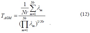
If T_AGM>γ_AGM , then there are PUs in the space, and vice versa. γ_AGM represents the detection threshold of the arithmetic-to-geometric (AGM) algorithm.

5) Eigenvalue Energy Summation

The eigenvalues of the received signal covariance matrix can represent the energy of the signal. We perform energy summation of the eigenvalues and extract a root to find its amplitude, written as:

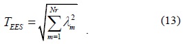
If T_EES>γ_EES , then there are PUs in the space, and vice versa. γ_EES represents the detection threshold of the eigenvalue energy summation (EES) algorithm.

6) Double Maximum Eigenvalue Detection

Under a binary hypothesis, H₀ indicates that no PUs exist, and thus while H₁ indicates the opposite and thus This algorithm is similar to the MED algorithm, but instead of the maximum eigenvalue, the sum of the two largest eigenvalues is used. The detection statistic can then be written as follows:

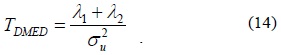
If T_DMED>γ_DMED , then PUs exist in the space, and vice versa. γ_AGM represents the detection threshold of the double maximum eigenvalue detection (DMED) algorithm.

7) Eigenvalue Weight

The eigenvalues of the received signal covariance matrix reflect its projected length in the direction of the eigenvectors to some extent, which is also the energy of the signal in this direction. Thus we consider making full use of this property of the eigenvalues, taking a proportion of the energy of each signal in the received signal as a weighted value, and the weighted energy as the detection threshold:

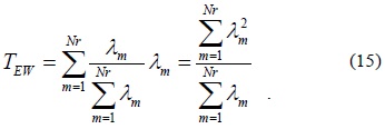
If T_EW>γ_EW , PUs exist in the space, and vice versa. γ_EW represents the detection threshold of the eigenvalue weight (EW) algorithm.

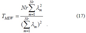
8) Multiple Eigenvalue Weight

For the eigenvalues of the received signal, we can conclude that

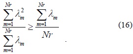
where the left part of the inequality is the detection statistic of the EW algorithm. If the right part of the inequality is shifted to the left, and the new detection statistic is expressed as

If T_MEW>γ_MEW , PUs exist in the space, and vice versa. γ_MEW represents the detection threshold of the multiple eigenvalue weight (MEW) algorithm.

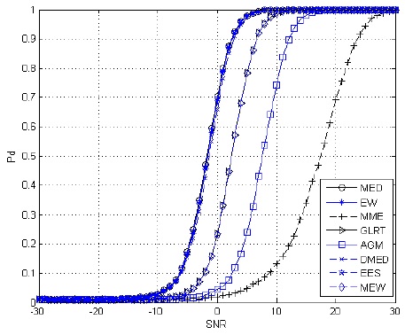
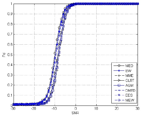
In this paper, we suppose that the SU’s receiver has 4 antennas, D—the number of PUs in the space—is smaller than 4, and the transmitting signal of the PUs is binary phase shift keyed (BPSK). Meanwhile, we assume that the channels between the PUs and the SUs are Rayleigh channels. We initialize the false alarm probability as 0.01. For the number of sampling points, we set 3 values, N=4, N=8, and N=100, and compare the performance of each algorithm with each number of sampling points. All the results are averaged over 10,000 Monte Carlo realizations.

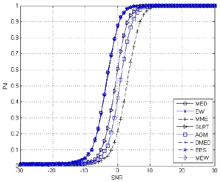
From the simulation results shown in Figs. 2–4, we can conclude the following.

When there is only one PU in the environment, as the number of sampling points N increases, the detection performance of each algorithm improves as well. The performance of EW, MED, DMED, and EES are better; GLRT, MEW, and AGM are ordinary; and MME performs the worst. Because of the existence of only one PU, eigenvalues are noise variance except for the maximum eigenvalue. The weight of the maximum eigenvalue in EW is approximately 1, and the second eigenvalue of DMED is noise variance, which can be ignored, as can be the energy of the noise component in EES. Thus the performance of these three algorithms are virtually the same as MED. MED and DMED are half-blind algorithms, since they both require noise information, while EW and EES are blind algorithms since they need no noise information and are not affected by noise. To sum up, EW is more practical in this case.

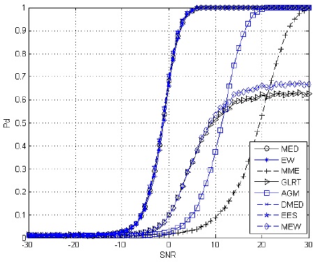
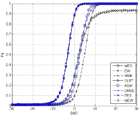
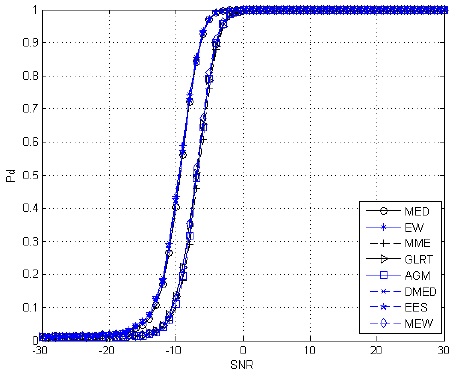
From the simulation results shown in Figs. 5–7, we can conclude the following.

When there are two PUs in the space, as the number of sampling points N increases, the detection performance of each algorithm improves as well. The performance of EW, MED, DMED, and EES are better; AGM is ordinary; and MME performs the worst. When N is 4, GLRT and MEW perform badly. The detection probability can only reach about 0.65. When N increases, the performance of these two algorithms improves.

Regardless of whether one or two PUs are in the environment, the EW algorithm has favorable detection performance under a low SNR. For instance, when the detection probability comes to 0.6 and N=4, the perfor-mance gain of the EW algorithm is 21 dB higher than that of the MME algorithm, and 9 dB higher than that of the AGM. This algorithm is suitable for a situation in which the PU’s signals are unknown, the signal energy is inferior and the existence of the PUs needs to be quickly detected.

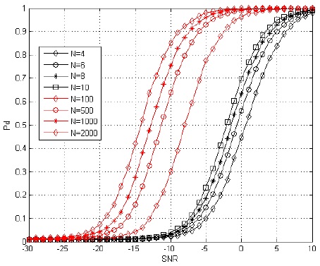
From the simulation result shown in Fig. 8, we can conclude the following.

For the EW algorithm, as the number of sampling points N increases, the detection performance improves as well. When the detection probability is 0.6 and the number of sampling points is smaller than 10, as the detection performance increases by one decibel, the number of sampling points increases by only 2 points. When the number of sampling points is larger than 500, as the detection performance increases by a decibel, the number of sampling points increases by about 500 points, and this demand will greatly increase as the number of sampling points increases. Thus, the EW algorithm can meet the requirements consistently and effectively under the conditions in which the signal and noise information is unknown, high system detection performance is needed, and the detection has to be implemented quickly.

This paper has proposed various new spectrum-sensing algorithms based on the joint distribution of the eigenvalues in a multiple-user cognitive radio environment, which make full use of the impact of the eigenvalue component during detection, acquire favorable detection performance under a low SNR, and ensure the robustness of detection with a small number of sampling points. In a study to follow, we plan to analyze the proposed algorithms theoretically on the basis of RMT.