There is the possibility that an ion trap mass spectrometer incorporates such traps as the Penning,1 Paul2 or Kingdon3 traps. In 2005, the Orbitrap was introduced according to the Kingdon trap.4 The two most popular kinds of ion traps are the Penning and the Paul traps (quadrupole ion trap).5-8 Of course, it is also possible that other kinds of mass spectrometers utilize a linear quadrupole ion trap selected as a mass filter. Interestingly, ion trap mass spectrometry has undergone many developmental stages in order to achieve its current condition with relatively high performance level and growing popularity. Paul and Steinwedel9 invented Quadrupole ion trap (QIT) commonly used in mass spectrometry,5-8 ion cooling and spectroscopy,10 frequency standards,11 quantum computing12 and others. However, different geometries have also been suggested and utilized for QIT.13
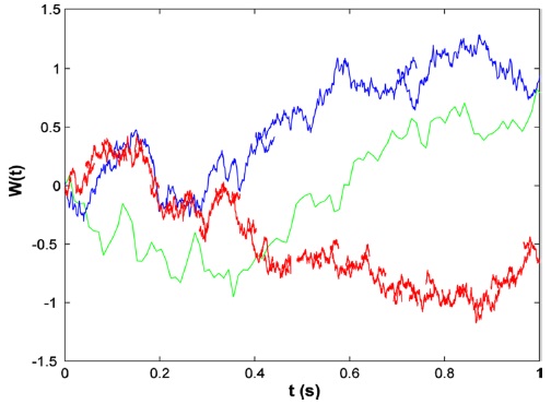
Main properties of Wiener process
A Wiener process14,15 (notation
Main properties of
•
• Trajectories of Wiener process are continues functions of
• expectation
• correlation function
• for any
• for any
• Increments of Wiener process on non overlapping intervals are independent, i.e. for (
• paths of Wiener process are not differentiable functions,
• martingale property,
>
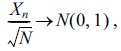
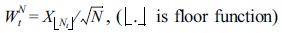
Wiener process as a scald random walk
Consider a simple random walk

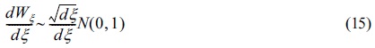
where {

in distribution as
In can be shown that as
The motions of ion inside quadrupole ion trap with stochastic potential form
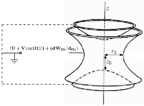
Fig. (2) shows indicatesa the schematic perspectives of a quadrupole ion trap (QIT). The quadrupole ion trap is the ion trap which including hyperbolic geometry and also is composed of involves a ring and two end cap electrodes that facing face each other in the

Where

Here,

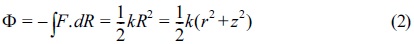
As Eq. (2) is unable to satisfy the Laplace situation, thus for confining the ions in two dimensions, it seems to be necessary to use a complicated potential as follows,

For satisfying Eq. (4), in a Laplace situation, ∇2Φ=0, the following equations are required,

This possibility is generated via four hyperbolic electrodes. In order to achieve such type of electrodes, the surfaces can be considered with the same potential Φ0/2 and –Φ0/2, as follow,

These situations make us able to find, and therefore Consequently, electrodes shaped for the potential (4) can be obtained as follows,
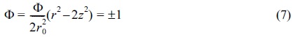
Eq. (7) represeznts a hyperbolic equation for this potential. Also, the potential Φ0 used in hyperbolic electrodes is as follow,

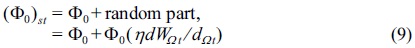
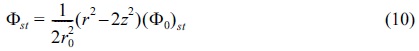
thus, the stochastic potential, (Φ0)

where
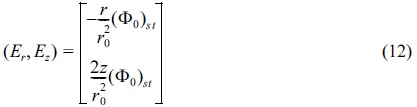
field elements in the trap therefore becomes,

Where ∇ is the gradient. From Eq. (11) we obtain,

The equations of motion for a singly charged positive ion in the QIT is represented thusly,
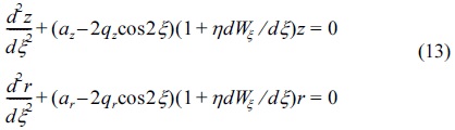
The
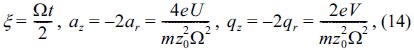
where
Thus, Ω/2

here,
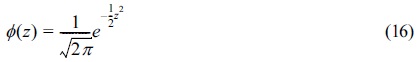
In Matlab, the command “randn” was used to add the elements of distribution
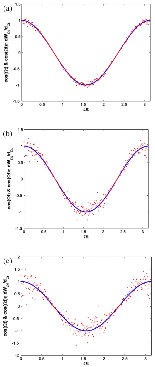
Fig. (3) compares the periodic impulsional potential of the form
Two stability parameters monitor the ion motion for each dimension
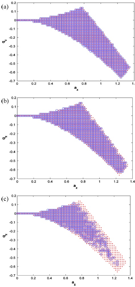
Fig. (4) displays the calculated first stability area for the quadrupole ion traps including and excluding the stochastic potential, red points (red color): QIT, blue circles (blue color): stochastic QIT, (a):
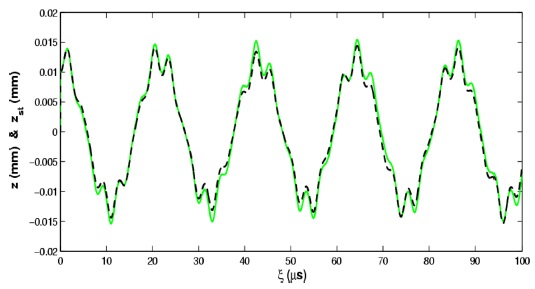
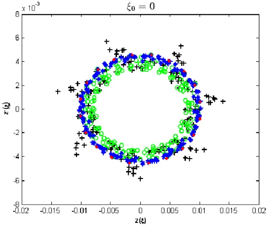
Fig. (5) indicates the ion trajectories in real time for stochastic as well as deterministic cases including
From a mathematical viewpoint, stochastic as well as theoretical results are closely related. Thus, employing stochastic procedure in quadrupol ion trap potential makes us able to simulate and obtain the numerical outcomes including high accuracy (see Figs. (5)). Table (1) reveals the values of

Here is the mean of
Table (1) indicates the values of
The values of
Table (3) represents the values of
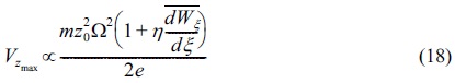
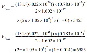
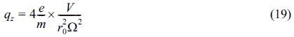
Now, we use Eq. (19) to calculate

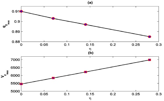
Fig. (6A) shows the behavior of function
Fig. (6B) shows
>
The effect of stochastic potential form on the mass resolution
Generally, the resolution of a quadrupole ion trap mass spectrometry21 can be regarded as a function of the mechanical precision of the hyperboloid of the QIT Δ
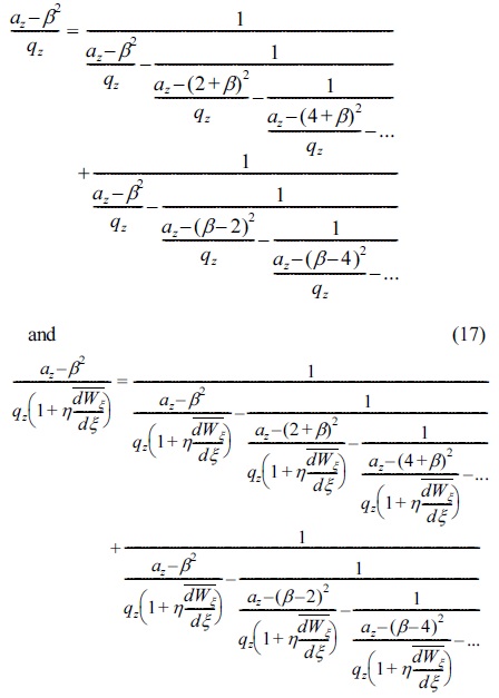
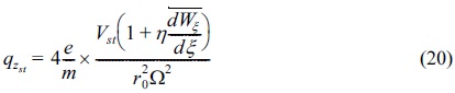
For deriving an influential theoretical formula for fractional resolution, we should consider the stability parameters of the impulse excitation for the QIT including and excluding its stochastic potential, respectively as follows,
By taking the partial derivatives associated with the variables of the stability parameters
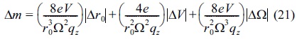
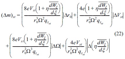
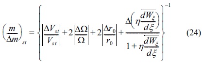
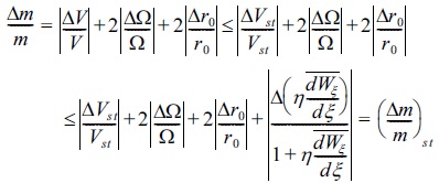
Now, in order to find the fractional resolution, we have,
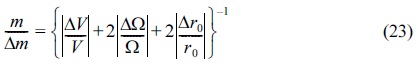

here Eq. (24) and Eq. (25) are the fractional resolutions for QIT with and without stochastic potential, respectively.
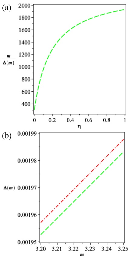
Fig. (7a) indicates the fractional resolution that is a function of the noise coefficient
Regarding the fractional mass resolution, the following uncertainties were used for the voltage, rf frequency and the geometry; Δ
Theoretically, we have,

Thus, (
Fig. (8) indicates the evolution of the phase space ion trajectory for different values of the phase
The results represented in Fig. (8) indicates that for the same equivalent operating point in the two stability diagrams (having the same
From a mathematical point of view, the results of stochastic process has higher resolution during mass separation. It has been shown that (
All authors read and approved the final manuscript.
The authors declare that they have no competing interests.