Obstacles in a maritime scenario can be big cargo ships, vessels, yachts, and/or small buoys. Successful detection of these obstacles provides important information for either navigation or object detection and the tracking of unmanned surface vehicles (USVs) [1-3]. The methods for obstacle detection in maritime images can be roughly categorized into two-dimensional (2D) image-based and three-dimensional (3D) stereo vision-based methods. The 3D methods [4,5] use two stereo images to obtain a 3D point cloud of the scene, which is then applied to fit the sea surface plane and cluster the points above this plane as obstacles. The 2D methods can either use graphic models to separate the sky, horizon, and sea areas and then segment the obstacles from the sea area [6], or apply saliency detection to estimate the obstacles [7]. In this work, we use a 2D image-based method because of the low camera budget and the relatively small computational burden.
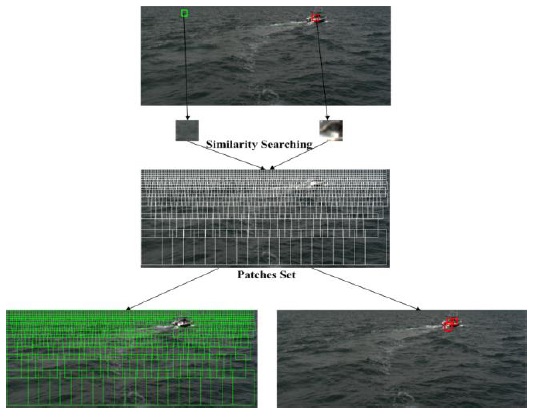
Sparsity potential (SP), originally proposed in [8] for object detection, is a measure that captures the sparseness or similarity of an image patch with respect to its neighborhood. In [8], image patches with a high value of SP are considered to be more discriminative and chosen for training and testing with Hough Forests. However, there are some limitations of applying such a local SP to maritime images because of the unique properties of a sea surface. For example, the neighboring patches of an image patch of the top of a sea wave may contain the bottom of the sea wave; thus, the image patch in the center would be highly distinct from its neighbors and have a low self-similarity or SP value, which would lead to a high probability of being classified as a patch of obstacles. In contrast, if the image patch is sampled from a big cargo ship, it may have a very similar appearance to its neighboring patches; this may lead to a high SP value, and the image patch may be wrongly classified as the background. Therefore, to reduce the abovementioned detection error in maritime images, we propose “global sparsity potential (GSP)”, which computes the self-similarity of an image patch within the entire sea surface area. By taking into account the entire sea surface area, we find that the image patch on the sea has more similar patches in the entire set of patches, while the image patch on the obstacles has the opposite. Thereafter, the discriminative power of image patches increases, and it becomes easier to separate the foreground (obstacles) patches from the background (sea) ones. As illustrated in Fig. 1, one can see that compared to the patch of obstacles, which only has three similar patches in the patch set, the patch of the sea is considerably less sparse and more similar to most of the patches.
In [9], the researchers proposed the use of variable-size image windows and feature space reclustering for detecting obstacles in maritime images. In their work, an iterative reclustering method is proposed to determine the centroid of the main cluster (sea), whose outliers are considered obstacles. Nevertheless, the clustering process in this method is sensitive to the outliers in the computation of the mean or the median of the feature set, thus leading to poor performance when there are a larger number of obstacles or more white wake outliers in the image. To solve this problem, in this study, we omitted the reclustering process and used GSP for estimating the mean feature of the sea. Then, as in [9], the outliers were considered obstacles.
In summary, two contributions are made in this paper. One is that we introduce a new measure, GSP, to represent the sparseness of an image patch with respect to the entire sea surface area. The other is a novel image-based obstacle detection algorithm using GSP for USVs; this algorithm has been experimentally proven to be more accurate and robust than the traditional method [9] and the state-of-the-art saliency detection method [10].
The rest of this paper is organized as follows: Section II introduces the proposed GSP measure and the proposed algorithm for obstacle detection in maritime images. Section III presents the experimental results with our own dataset and a comparison with other related work. Finally, Section IV concludes this work and discusses the future work in this area of study.
To ensure that only the sea surface area is processed and the sea surface is the dominating cluster, the proposed algorithm for maritime obstacle detection is based on two assumptions:
Therefore, only the obstacles below the horizon line in the images are considered the detection targets. In general, the proposed algorithm can be divided into three procedures: horizon detection, sampling and representation of image patches, and obstacle detection using GSP.
In [11], four different horizon detection methods were compared and analyzed, and it was concluded that the Random Sample Consensus (RANSAC) method provides the best results with high accuracy. Therefore, in this work, we apply the RANSAC method for horizon detection. To reduce the computational expense and the noise effect, it is usually better to set a region of interest (ROI) that contains the horizon. However, rather than predefine a fixed ROI for every frame as in [11], we propose a more general method to adaptively estimate the ROI.
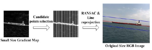
We first resize the original image to a smaller size (e.g., 64×64 in this work), because downsampling eliminates a considerable amount of noise, and the horizon can still be roughly estimated without significantly biasing the ground truth. In the downsized image, shown in Fig. 2, first, the gradient map is computed using a Sobel operator, and then, locations with the maximum gradient values along each sampled column are selected as the candidate points; RANSAC is used by randomly selecting two candidate points at each iteration to fit the horizon line. Finally, after reprojecting the estimated horizon in the small image onto the original image, we can define the ROI in the original image by moving the horizon vertically up and down for the same distance to form the upper and lower boundaries, respectively. Thereafter, RANSAC is used again as in [11] in the ROI for estimating a more accurate horizon in the original image.
As shown in Fig. 3, after the detection of the horizon line, the ROI for obstacle detection can be obtained via affine transformation and cropping. Then, further processing is performed on the ROI.
>
B. Patch Sampling and Representation
In 2D images, considering the geometric relation between the camera and the sea surface, the resolution of the observation that is close to the horizon is smaller than that of the observation close to the image bottom. Similar to [9], here, square image patches are sampled from the ROI by using variable-size image windows with an overlap rate of
To represent the abovementioned sample patches, we adopt a gray-level co-occurrence matrix-based texture analysis [12] as in [9]. In this method, all patches are first resized to the same size (


where
>
C. Obstacle Detection Using GSP
Here, we denote an image patch with a feature vector expression as
1) Measure of GSP
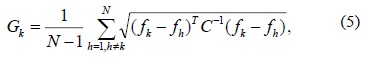
In this work, the GSP of an image patch is measured by its global self-similarity, which computes the similarity of a query patch to the entire patch set. Different from [13], which extracts the global self-similarity descriptors by performing a cross correlation of the patches in the entire image for object classification and detection, we measure the texture similarity of a query patch to the entire patch set by respectively computing their Mahalanobis distances. The smaller the distance between two patches, the higher is the similarity between them. Then, all the computed distances to the patch set are summed and their average is taken as the global self-similarity measure of this query patch. Eq. (5) formulates the global self-similarity

where
2) Clustering of Features
In [9], the centroid of the main cluster (sea) is estimated using an iterative procedure. However, this method may be sensitive to the outliers, because at each iteration, it treats all image patches equally in order to compute the mean or median feature. Therefore, including these outliers in the estimation of the centroid of the sea may decrease the accuracy. In this work, to overcome the abovementioned drawback, we propose to select image patches with a high probability to be a sea surface, i.e., having a relatively low GSP value, to estimate the centroid (mean feature) of the sea. Thereafter, the procedure for feature clustering can be summarized as follows:
Since there are few available public datasets for maritime obstacle detection, we built our own dataset, the details of which are described in Section III-A. Using this new dataset, we evaluated the accuracy of the proposed algorithm and compared its performance with that of the traditional method [9] and that of a state-of-the-art saliency detection approach [10] in Section III-B.
Our maritime obstacle detection dataset consists of four sequences (S_#1, S_#2, S_#3, and S_#4), which were captured by a Point Grey grasshopper CCD camera mounted on a moving USV on the sea. Each sequence contains 600 RGB frames (size: 684×548 pixels). The obstacle in this dataset is a moving target boat, which varies its distance (approximately from 50 m to 500 m) to the USV (camera boat). The different sequences present different challenges:
S_#1 characterizes the detection ability for a short distance, in which the target boat moves close to the USV (within 100 m);
S_#2 contains many white wake outliers generated by the fast moving target boat, and the distance is around 100 m to 200 m.
S_#3 has a majority of the frames without the obstacle shown, and the target boat quickly moves 200 m away from the USV, and from the left to the right of the image in a few frames at the middle of the sequence; this also provides some white wake outliers.
S_#4 renders the challenge of distant obstacle detection, and the target boat moves a distance of 200 m to 500 m away.
Since the proposed algorithm is based on the prior knowledge of the horizon line, only images whose horizons are detected can be processed for the obstacle detection. Thus, images without a detected horizon are discarded, and not considered in the accuracy or the false rate calculation of the obstacle detection.
The parameters for variable-size windows in the image patch sampling part are set as follows: overlap rate
Similar to [14], the accuracy evaluation is performed visually as follows:
Integrating the two above-discussed cases, we can express the score assigned to
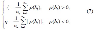
Finally, as formulated in (7), the detection accuracy

where
Table 1 summarizes the performance of obstacle detection using the proposed algorithm and two comparative algorithms.
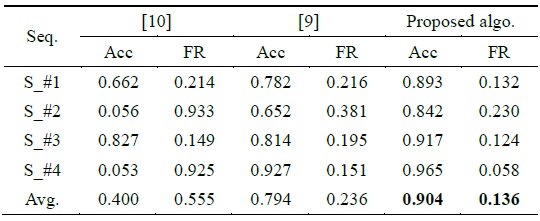
Comparison of accuracy (Acc) and false rate (FR) for maritime obstacle detection using different methods
The main difference between the proposed algorithm and the feature space reclustering method [9] is the computation of the centroid of the sea features. In [9], the authors proposed the use of all the features of the sampled image patches to estimate the centroid iteratively, while our method involves the selection of image patches with small values of GSP and the calculation of their mean to estimate the centroid. Theoretically, the proposed algorithm is more insensitive to the outliers of the sea features, because rather than taking all the features, which may contain many outliers, to compute the mean or median feature, we just use features with high probabilities to be the sea to compute the mean feature. We reimplemented the method of [9] with the same parameter settings for variable-size window sampling and feature extraction on our maritime obstacle detection dataset. Experimental results show that the proposed algorithm is more accurate than that proposed in [9].
As shown in Table 1, the accuracy of the proposed algorithm is more than 10% compared to that proposed in [9] in the first three sequences, which contain many outliers caused by the white wake. Nevertheless, in sequence S_#4, our method performs only slightly better than that proposed in [9]. This could be attributed to the fact that the obstacles in most frames of S_#4 are far away from the camera, so there are very few outliers, such as white wake, in the images. Fewer outliers lead to more accurate estimation of the centroid of the sea; thus, only a small accuracy gap exists between our method and that proposed in [9]. In addition, our method exhibits a smaller false detecting rate than that proposed in [9].
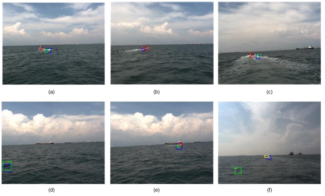
Some advantages of the proposed algorithm over the method proposed in [9] can be seen in Fig. 4. In Fig. 4(a) and (c), false detection caused by white wake happens in the case of the method proposed in [9]. In Fig. 4(f), the method proposed in [9] has two detections, in which one is correct and the other is false and is caused by a sea wave; the same false detection is also observed in the scenario of Fig. 4(d). Only a small portion of the boat is detected by the method proposed in [9] in Fig. 4(e), and this situation is classified as
To test the saliency detection method for our task, we implemented the work of [10] with our own dataset. As shown in Table 1, however, this state-of-the-art method for saliency detection does not perform well for our dataset. However, intuitively, it seems that the obstacles on the sea are more distinct and salient than the sea water. In fact, the saliency-based methods, which usually use the image local contrast information to detect distinct regions, are sensitive to the sea wave. For example, it can be seen in Fig. 4(a), (b), (c), and (f) that the white wake generated by the boat causes a big problem for this saliency detection method, which results in many false detections. Similarly, in Fig. 4(d), the dark region between the wave top and the wave bottom is detected as the saliency, but this region is not an obstacle. Although the detected saliency in Fig. 4(e) contains the obstacle, the bounding box is very big and is not well-fitted to the obstacle. Therefore, we can conclude that it may not be a wise choice to only apply saliency detection to solve the maritime obstacle detection task.
In this paper, we introduced a new measure, “global sparsity potential (GSP)”, to capture the sparseness of an image patch throughout the sea area. Using GSP, we developed an accurate and robust approach for moving camera-based obstacle detection in maritime images. In this approach, image patches with a relatively small GSP value are considered the main cluster (i.e., sea surface), while their outliers, which have a relatively large GSP value and a relatively large Mahalanobis distance with respect to the mean feature of the sea surface), are considered the obstacles.
Although the proposed algorithm exhibits good performance, only the intensity image and the texture feature are explored. Further improvements can be expected by combining the color information and other discriminative features in a future work.


![Superior performance for maritime obstacle detection of the proposed algorithm (red) compared to that of the method of feature space reclustering [9] (green) and that of saliency detection VOCUS2 [10]. The yellow bounding box in (f) means that the red and the green bounding boxes are overlaid. (a) and (b) are from S_#1; (c) is from S_#2; (d) and (e) are from S_#3; and (f) is from S_#4. One can see that the performances of these three methods can be easily evaluated by human eyes.](http://oak.go.kr/repository/journal/20511/E1ICAW_2016_v14n2_129_f004.jpg)