Modelling and Simulation Resolution of Ground-Penetrating Radar Antennas

Alsharahi
						G.; Mint Mohamed Mostapha
						A.; Faize
						A.; Driouach
						A.

doi:10.5515/JKIEES.2016.16.3.182

OA학술지
Journal of electromagnetic engineering and science

Modelling and Simulation Resolution of Ground-Penetrating Radar Antennas

DOI : 10.5515/JKIEES.2016.16.3.182
Author: Alsharahi G., Mint Mohamed Mostapha A., Faize A., Driouach A.
Publish: Journal of electromagnetic engineering and science Volume 16, Issue3, p182~190, 31 July 2016

ABSTRACT

The problem of resolution in antenna ground-penetrating radar (GPR) is very important for the investigation and detection of buried targets. We should solve this problem with software or a numeric method. The purposes of this paper are the modelling and simulation resolution of antenna radar GPR using three antennas, arrays (as in the software REFLEXW), the antenna dipole (as in GprMax2D), and a bow-tie antenna (as in the experimental results). The numeric code has been developed for study resolution antennas by scattered electric fields in mode B-scan. Three frequency antennas (500, 800, and 1,000 MHz) have been used in this work. The simulation results were compared with experimental results obtained by Rial and colleagues under the same conditions.

KEYWORD

Antenna , FDTD , GPR , Modelling , Simulation , Resolution

본문

Collapse all

I. INTRODUCTION

Ground-penetrating radar (GPR) is an electromagnetic survey widely used in non-destructive resolution studies. This method has one of the highest resolutions in subsurface imaging of any non-invasive geophysical method [1].

Numerical modeling and simulation of GPR signals are widely used and have been recognized as the best way to achieve our results. A variety of differential equations and integral equations based on numerical modeling techniques have been developed for this purpose [3, 4]. This research intends to highlight these issues by incorporating a finite-difference time domain (FDTD) simulation for several cases. When applying the FDTD method in GPR simulation using REFLEXW, the permittivity and the electromagnetic wave attenuation are the most important parameters of the medium that should be taken into consideration for the GPR method. The GPR reflection profiling entails simulation movement of both the transmitting and receiving antennas along the profile line [4]. Radar is used to detect an object based on radio waves. This method is based on the emission of very short time domain electromagnetic pulses. Spatial resolution depends on the characteristics of the radar signal, the survey, the electromagnetic (EM) properties of the studied medium, and the distance of the antenna to the target. The frequencies, the number of scans over the target, and the spatial antenna beam pattern are the features defining the radar signal and the survey [5]. The resolution of subsurface features is partly affected by antenna wavelength, which is also directly related to the frequency for higher frequency radar, providing higher resolution than a lower frequency radar [2, 10].

The simulation was compared to the data of an experimental work [6], and the results showed a good performance. In particular, this work deals with the development of a set of simulations in order to analyze the resolution capacity of three bow-tie antennas at frequencies of 500, 800, and 1,000 MHz, simulating with their real resolution capacity and comparing it with the theoretical. This paper focuses on the methodology proposed to carry out the antenna resolution. These simulations are carried out in the air using two timber structures designed and constructed for this purpose.

II. METHODOLOGY

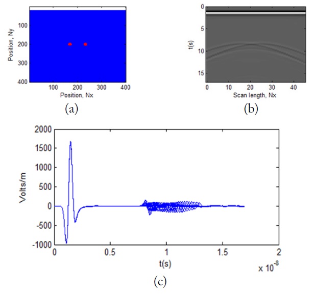
In this work we distinguish between buried objects of the same type and geometrics shape by simulation thus comparative with to the experimental work published by Rial et al. [6], who used the same objects: a rectangular wood bar (2 cm × 4 cm) and a metallic circular bar (radius = 2 cm) buried in a medium of air. They have the physical properties shown in Table 1. We will simulate the resolution of the GPR antenna in the medium of dry sand using GprMax2D in time and a frequency domain of 800 MHz.

[Table 1.] Physical properties of the materials

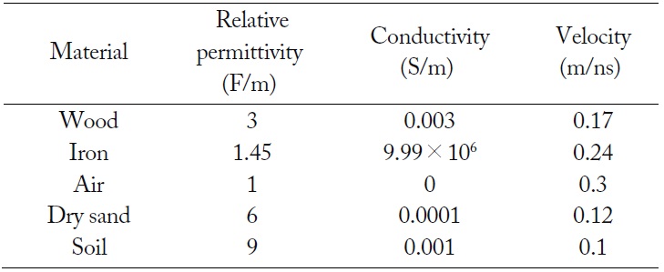
Physical properties of the materials

   1. Description of Software

- REFLEXW software: In what follows, we discuss the description of the software REFLEXW, whose algorithm is based on the FDTD. This software is designed to process the signals taken from the subsoil radar [11-16].

- GprMax2D/3D: GprMax is based on FDTD and is available free of charge for both academic and commercial use; it has been successfully employed in situations. The tool can be downloaded from www.gprmax.org or by contacting the author [17].

   2. Description Antennas

2.1 Antenna Arrays

Two types of antenna arrays are taken into account: antenna transmitter and receiver (ATR): x-, y-coordinates, angle, and frequency for both transmitter and receiver. The x-coordinate will be added to the profile constant start coordinate given in code AM, and the y-coordinate will be added to the profile start coordinate given in code FX, in this work has used in REFLEXW. The wave used in this antenna is Kuepper, sinusoidal, and continuous.

2.2 Antenna Dipole

The antenna dipole consists of two identical conductive elements, such as metal wires or rods, which are usually bilaterally symmetrical. The driving current from the transmitter is applied, or, for receiving antennas, the output signal to the receiver is taken between the two halves of the antenna. The wave used in this antenna will be Ricker or Gaussian along the length of the dipole as used in GprMax2D.

Dipoles mounted horizontally (as is more common) will have gain in two opposing horizontal directions, but nodes (directions of zero gain) will be at 90° from those directions (along the direction of the conductor).

A half-wave dipole antenna consists of two quarter-wavelength conductors placed end to end for a total length of approximately L = λ/2.

2.3 Bow-tie Antenna

This antenna will have a similar radiation pattern to the dipole antenna, and it will have vertical polarization. A L = 76.5 mm bow-tie antenna with a width of W = 36 mm, (so that the angle D = 2 × atan(76.5/36) = 130°). The separation between transmitting and receiving antennas (S_TxRx) and typical geometries of these antennas and their physical dimensions are shown in Table 2.

[Table 2.] Geometries and dimensions of 500, 800 and 1,000 MHz GPR antennas

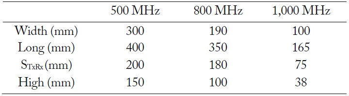
Geometries and dimensions of 500, 800 and 1,000 MHz GPR antennas

III. BACKGROUND THEORY

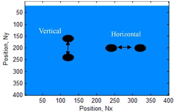
The vertical resolution is nothing other than the smallest difference in time between two objects of the same type; the GPR can distinguish them. We can then say that vertical resolution is the smallest distance; this is the direction perpendicular to the surface that two targets can be apart for us to see them and distinguish them as separate objects. The horizontal resolution is a bit clearer because distance is measured in the length units and not in the time units. So, the horizontal resolution is the minimum distance between two objects in the same horizontal plane parallel to the surface where the radar “sees” both objects as separate [7, 14].

   1. Modelling based on the FDTD Method

Maxwell’s equations in electromagnetic fields describe the electric and magnetic fields arising from distributions of electric charges and currents. They can be used to describe all the electromagnetic fields; the propagation of electromagnetic fields is governed by Maxwell’s Eqs. (1a)–(1c),

where is the magnetic flux density in V · s/m²,

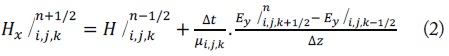
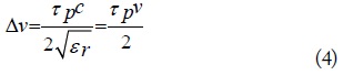
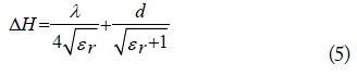
This equation calculates the field E_yⁿ⁺¹ based on field The same procedure is followed for the expression of each component of the electromagnetic field. This discretization of Maxwell’s equations constitutes the basis of the Yee algorithm. For the TE mode, the 2D FDTD equations become [19]:

   2. Resolution

The accuracy of an antenna is in the antenna’s ability to detect and distinguish between two or more targets separated by a horizontal or vertical distances, as shown in Fig. 1. The horizontal resolution of the antenna is based on the presentation package antenna radiation and wavelength, as shown in Eq. (5), when the bandwidth, the narrow horizontal of the antenna, gives the best accuracy. Furthermore, the vertical resolution is strongly affected by the duration of the pulse radar and the central frequency of the antenna. The vertical resolution can be calculated by Eq. (4), from the effective duration τ_P of the radar pulse, as shown in Table 3, and the wave propagation velocity v(m/ns) in the medium vertical resolution [8, 9, 11].

[Fig. 1.] Vertical and horizontal resolution diagram.

[Table 3.] Effective pulse duration and central frequency for the 1,000, 800, and 500 MHz antennas

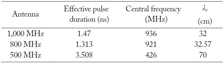
Effective pulse duration and central frequency for the 1,000, 800, and 500 MHz antennas

The horizontal resolution can be calculated by

where λ is the wavelength and d is depth.

   3. Beam Width

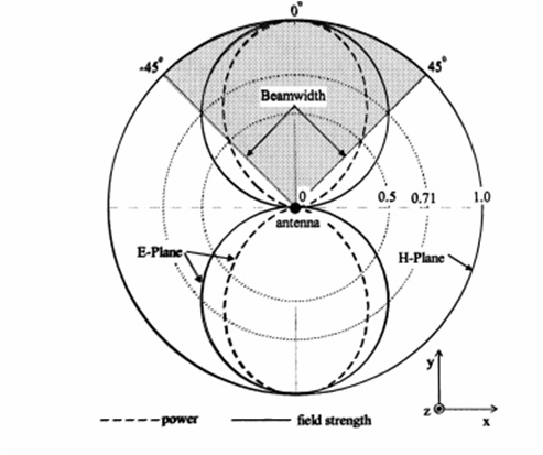
The theoretical relative field and power patterns of a short dipole antenna are shown in Fig. 2. The two points of about 71 % of the maximum point in the field pattern or 50% of the maximum point in power pattern are commonly used to mark the beam width of the antenna radiation. Since in practice the difference between the maximum and minimum values is very large, it is common to express the measured relative power in decibel (dB), defined as follows:

or

where P and E are the measured power and field strength, respectively, while P_max and E_max are the maximum values.

[Fig. 2.] Relative field and power patterns of a short dipole antenna.

The beam width of the antenna can be defined then by drawing two lines from the origin through the - 3 dB points as shown in Fig. 2 [18].

IV. RESULTS AND DISCUSSION

   1. Vertical Resolution

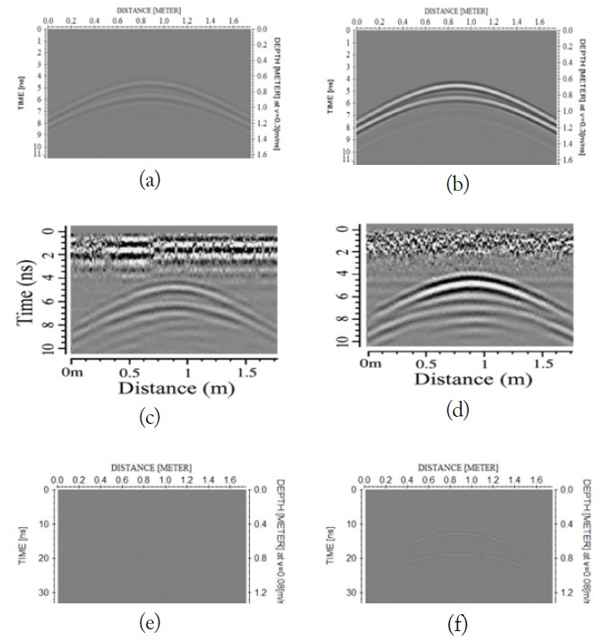
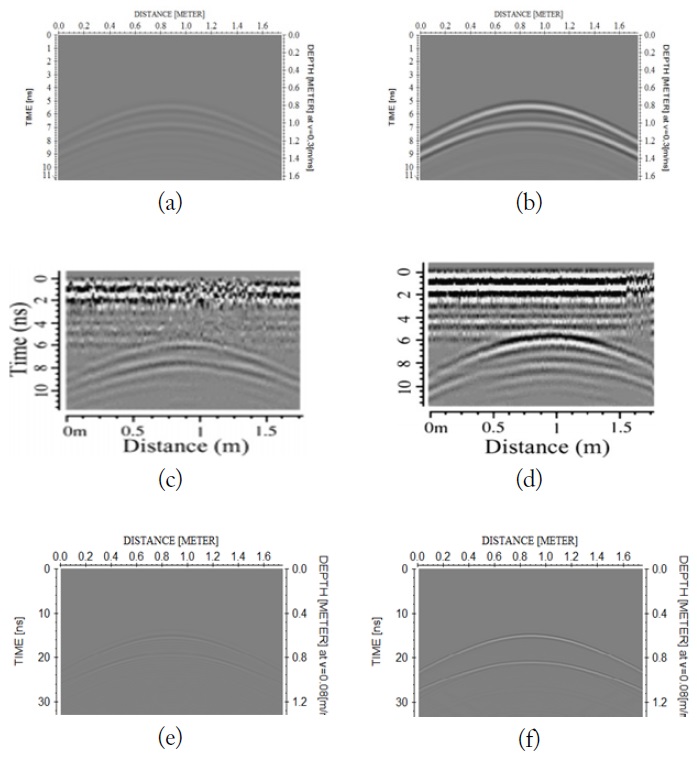
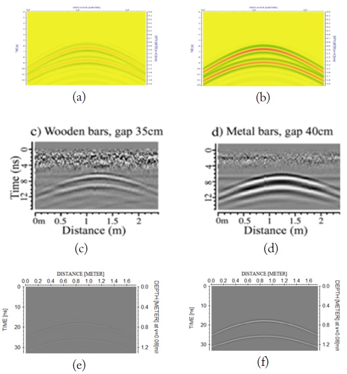
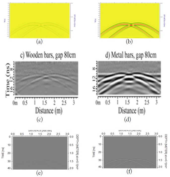
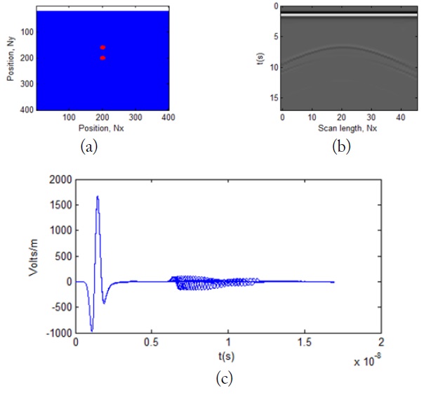
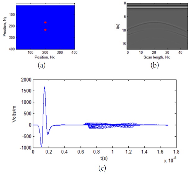
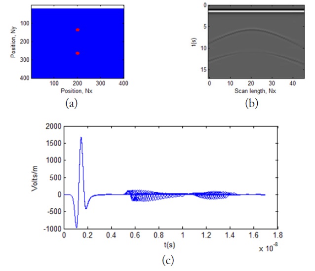
The results of the vertical resolution have been presented in Figs. 3-5. In Fig. 3(a), it is presented for wooden bars and in Fig. 3(b) for metal bars buried in mediums of air and soil. We note the presence of two hyperbolas that indicate the presence of the two bars at around 63 cm, as compared with experimental results [6] in Fig. 3(c) and 3(d) at 1,000 MHz. Fig. 4 shows two bars of metal and wood buried in the medium of air at a 74-cm depth with 800 MHz used; the bars are separated from each other with a distance equal to 20 cm. The simulation results of the vertical resolution at 800 MHz has compared with the experimental results [6] of Fig. 4(c) and 4(d). However, the results of our simulations seem to be the best. As expected, the vertical resolution was better for the higher frequency antennas because of their shorter pulse duration and was very similar for the 1,000 MHz and 800 MHz antennas. With regard to the different materials used in the simulations (wood and metal bars), the solution became worse when the metal bars were used, because of their higher electromagnetic contrast. A higher electromagnetic contrast decreases the energy of the signal received by the second reflector, so that a greater separation is necessary to detect discrete events. The type of materials is an important factor in estimating the vertical resolution of the two targets due to the fact that the materials that give a strong reflection are the most masking material that is near them and vice versa. Results obtained for the two antennas and measured vertical resolutions are summarized in Table 4, for the 800, 500, and 1,000 MHz antennas.

[Fig. 3.] Radargram simulation of vertical resolution at a 63-cm depth with a 1,000-MHz antenna. (a) Wooden bars simulation, 15 cm spacing; (b) metal bars simulation, 15 cm spacing; (c) wooden bars experiments, 20 cm spacing [6]; (d) metal bars experiments, 20 cm spacing [6]; (e) wooden bars buried in soil; and (f) metal bars buried in soil.

[Fig. 4.] Radargram simulation of vertical resolution at a 74-cm depth and a 800-MHz antenna. (a) Wooden bars simulation, 20 cm spacing; (b) metal bars simulation, 20 cm spacing; (c) wooden bars experiment, 20 cm spacing [6]; (d) metal bars experiment, 20 cm spacing [6]; (e) wooden bars buried in soil; and (f) metal bars buried in soil.

[Table 4.] Results of the vertical resolution (ΔV ) for the 1,000, 500, and 800 MHz antennas

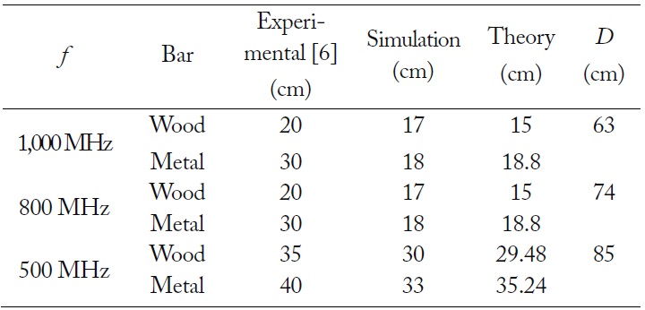
Results of the vertical resolution (ΔV ) for the 1,000, 500, and 800 MHz antennas

1.1 Vertical Resolution with the 1,000 MHz Antenna (Fig. 3)

1.2 Vertical Resolution with the 800 MHz Antenna (Fig. 4)

1.3. Vertical Resolution with 500 MHz Antenna (Fig. 5)

[Fig. 5.] Radargrams of the 500 MHz antenna with bars at 85 cm depth. (a) Wooden bars gap at 30 cm; (b) metal bars gap at 33 cm; (c) wooden bars gap at 35 cm. (d) Metal bars gap at 40 cm; (e) wooden bars buried in soil; and (f) metal bars buried in soil.

In this case, we show the 500 MHz antenna and different vertical distances, as shown in Fig. 5, in the mediums of air and soil.

1.4 Vertical Resolution by GprMax2d and Modelling in Dielectric Medium (800 MHz)

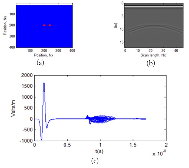
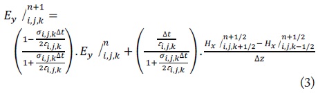
We will simulate for detection of a small bar of iron buried in a medium of dry sand, as shown in Fig. 6.

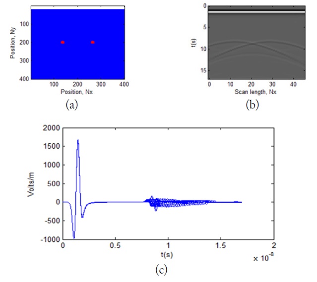
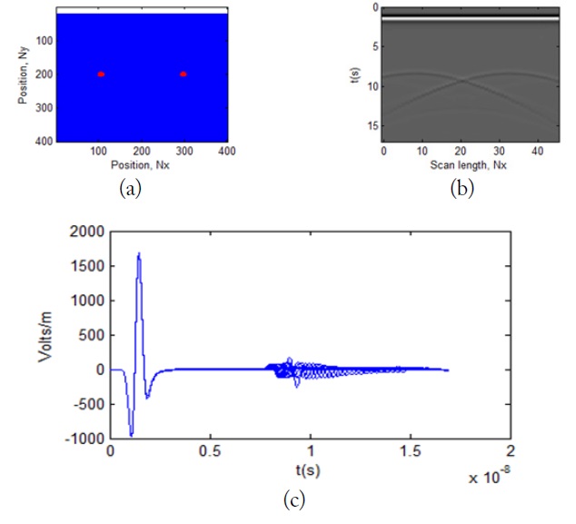
[Fig. 6.] Radargram simulation of detection for iron bar, 0.5 m depth at 800 MHz. (a) Schematic drawing of the targets buried; (b) radargram by GprMax2D; and (c) scattered electric fields from two targets in mode B-scan.

The results are difficult to distinguish between targets at a separation of 10 cm, as shown in Fig. 7(b). However, at a separation of 16 cm, we can distinguish between buried targets, as seen in Fig. 8(b) and Fig. 7(c), by signal. At a separation of 32 cm, it is very clear, as shown Fig. 9(b) and 9(c), by signal.

[Fig. 7.] Radargram simulations of vertical resolution, spacing 10 cm and 0.5 m depth at 800 MHz. (a) Schematic drawing of the targets buried; (b) radargram by GprMax2D; and (c) scattered electric fields from two targets in mode B-scan.

[Fig. 8.] Radargram simulation of vertical resolution, with a 16-cm spacing and a 0.5-m depth at 800 MHz. (a) Schematic drawing of the targets buried; (b) radargram by GprMax2D; and (c) scattered electric fields from two targets in mode B-scan.

[Fig. 9.] Radargram simulation of vertical resolution, spacing 32 cm and 0.5 m depth at 800 MHz. (a) Schematic drawing of the targets buried; (b) radargram by GprMax2D; and (c) scattered electric fields from two targets in mode B-scan.

   2. Horizontal Resolution

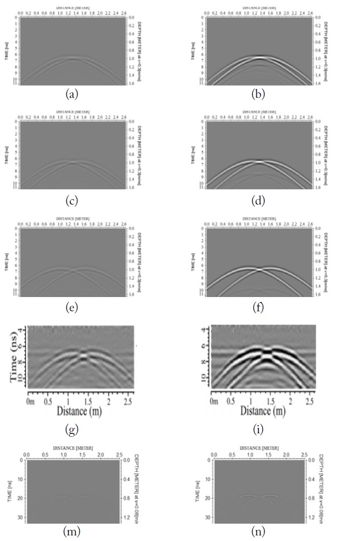
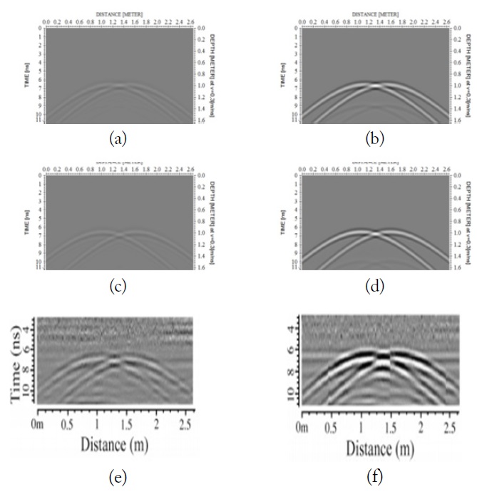
The frequencies of simulations were set at 800 MHz and 1,000 MHz. The results obtained are shown in Table 5 for the two antennas, and the measured horizontal resolutions were presented in Fig. 10 at 1,000 MHz and Fig. 11 at 800 MHz, using two rods separated horizontally by 20, 32, or 52 cm. Fig. 11(a), 11(c), and 11(e) show the results for wood bars, and Fig. 10(b), 10(d), and 10(f) show the results for metal bars. The results of horizontal resolutions are presented as shown in Fig. 10(e) at 1,000 MHz, and Fig. 11(f) at 800 MHz has compared with other results [6] in Fig. 10(g) and 10(i) for wood and metal bars, respectively. Fig. 11 used 800 MHz and a depth of 91 cm; the experimental results obtained from Rial et al. [6], as shown in Fig. 5(e) and 5(f), were compared to those from our simulation in Fig. 6(c) and 6(d). As expected, horizontal resolution worsens as the reflectors are moved away from the antennas, mainly because their footprint size gets larger. In radargrams of figures, the difference in the reflected signal for the two types of bars used during the tests can be seen. The influence of the type of bar in the resolution is less noticeable for the horizontal resolution than for the vertical one. This influence seems significant only when the bars are close to the antenna; then the hyperbolas become smaller and the wooden bars can be better distinguished. Results of horizontal resolution (ΔH) for the 1,000, 800, and 500 MHz antennas are shown in Table 5.

[Table 5.] Results of horizontal resolution (ΔH) for the 1,000, 800, and 500 MHz antennas

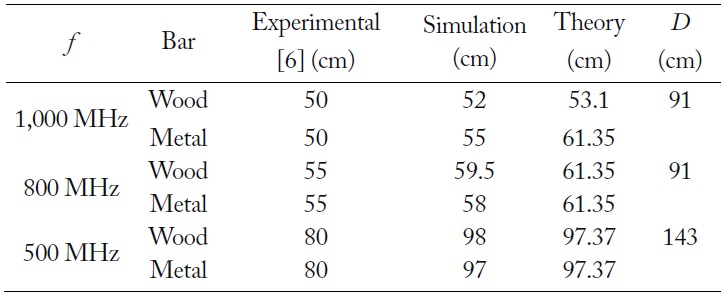
Results of horizontal resolution (ΔH) for the 1,000, 800, and 500 MHz antennas

[Fig. 10.] Radargrams simulation of horizontal resolution at a 91 cm depth with a 1,000-MHz antenna. (a) Wooden bars spacing 20 cm; (c) wooden bars spacing 32 cm; (e) wooden bars spacing 52 cm; (g) wooden bars experiments spacing 60 cm [6]; (b) metal bars spacing 20 cm; (d) metal bars spacing 32 cm; (f) metal bars spacing 52 cm; (i) metal bars experiments spacing 60 cm [6]; (m) wooden bars buried in soil; and (n) metal bars buried in soil.

[Fig. 11.] Radargrams simulation of horizontal resolution at a 91 cm depth and with a-800 MHz antenna. (a) Wooden bars spaced at 37.5 cm; (c) wooden bars spaced at 60 cm; (e) wooden bars experiments spaced at 60 cm [6]; (b) metal bars spaced at 37.5 cm; (d) metal bars spaced at 60 cm; (f) metal bars experiments spaced at 60 cm [6].

2.1 Horizontal Resolution with an Antenna of 1,000 MHz (Fig. 10)

2.2 Horizontal Resolution with a 800-MHz Antenna (Fig. 11)

2.3 Horizontal Resolution with a 500-MHz Antenna (Fig. 12)

[Fig. 12.] Radargrams of the 500 MHz antenna with bars at a depth of 143 cm. (a) Wooden bars with a gap of 98 cm; (b) metal bars with a gap of 97 cm; (c) experiment of wooden bars [6]; (d) experiment of metal bars [6]; (e) wooden bars buried in soil; and (f) metal bars buried in soil.

In this case, we use a 500-MHz antenna and different horizontal distances, as shown in Fig. 12, in the mediums of air and soil.

2.4 Horizontal Resolution by GprMax2D and Modelling in Dielectric Medium

Distinguishing between targets at a spacing of 10 cm is difficult in the results of the horizontal resolution, as shown in Fig. 13. At a separation of 16 cm, we can distinguish between buried targets, as seen in Figs. 13(b) and 14(c), by signal. At a separation of 32 cm, it is very clear (as shown in Fig. 15(b) and 15(c)) by signal.

[Fig. 13.] Radargram simulation of horizontal resolution, with a spacing of 10 cm and a 0.5-m depth at 800 MHz. (a) Schematic drawing of the targets buried; (b) radargram by GprMax2D; and (c) scattered electric fields from two targets in mode B-scan.

[Fig. 14.] Radargram simulations of horizontal resolution, with a spacing of 16 cm and a 0.5-m depth at 800 MHz. (a) Schematic drawing of the targets buried; (b) radargram by GprMax2D; and (c) time domain.

[Fig. 15.] Radargrams simulation of horizontal resolution, with a 20-cm spacing and a 0.5-m depth at 800 MHz. (a) Schematic drawing of the targets buried; (b) radargram by GprMax2D; and (c) scattered electric fields from two targets in mode B-scan.

However, when separated by 20 cm, we can distinguish between buried targets stronger than other cases, as seen in Fig. 16(b) and 16(c), by signal.

[Fig. 16.] Radargram simulations of horizontal resolution, with a 48-cm spacing and a 0.5-m depth at 800 MHz. (a) Schematic drawing of the targets buried; (b) radargram by GprMax2D; and (c) scattered electric fields from two targets in mode B-scan.

V. CONCLUSION

The radargrams were obtained by simulations using two different pieces of software, Reflexw and GprMax2D; they are perfect theoretically and more accurate than the results that have been obtained experimentally by GPR by Rial et al. [6] under the same conditions. The contribution in this work is a calculation of the resolution of antennas using a dispersion of the electric field that was successful and the use of several antennas. The vertical resolution of a GPR antenna can be better described described in terms of a distance equivalent to the center wavelength λ_c of the antenna. The resolution can also be represented by a distance equivalent to effective pulse duration τ_p, of the signal from the antenna. In air, the 800 MHz GPR antenna is a much better antenna. The vertical resolution of an antenna on dielectric can be adequately represented by a distance equivalent to one half (λ_c/2) of the center wavelength λ_c of the antenna in the respective medium. The amelioration in vertical resolution as compared to that in the air is probably due to the change in the signal waveform of the antenna. The horizontal resolution of the 800 MHz antenna on a dielectric will be suitably represented by the effective 3-dB beam width, 4BW of the antenna in the respective medium.

참고문헌

1. Daniels D. J. 2004 Ground Penetrating Radar.
2. Conyers L. B. 2004 Ground-Penetrating Radar for Archaeology.
3. Jol H. M. 2009 Ground Penetrating Radar Theory and Applications.
4. Czaja K. 2012 "Application of electromagnetic field modelling in GPR investigations of an historic tenement," [Geology, Geophysics and Environment] Vol.38 P.395-410
5. Perez-Gracia V., Di Capua D., Gonzalez-Drigo R., Caselles O., Pujades L. G., Salinas V. 2010 "GPR resolution in cultural heritage applications," [in Proceedings of 2010 13th International Conference on Ground Penetrating Radar (GPR)] P.1-5
6. Rial F. I., Pereira M., Lorenzo H., Arias P., Novo A. 2009 "Resolution of GPR bowtie antennas: an experimental approach," [Journal of Applied Geophysics] Vol.67 P.367-373
7. Cabrera R. A. 2007 GPR Antenna Resolution.
8. Perez-Gracia V., Gonzalez-Drigo R., Di Capua D. 2008 "Horizontal resolution in a non-destructive shallow GPR survey: an experimental evaluation," [NDT & E International] Vol.41 P.611-620
9. Perez-Gracia V., Gonzalez-Drigo R., Di Capua D., Pujades L. G. 2007 "Experimental analysis of the resolution in shallow GPR survey," [in Remote Sensing for Environmental Monitoring, GIS Applications, and Geology VII]
10. Davis J. L., Annan A. P. 1986 "Machinations: high-resolution sounding using ground-probing radar," [Geoscience Canada] Vol.13 P.205-208
11. Millard S. G., Shaari A., Bungey J. H. 2002 "Resolution of GPR bow-tie antennas," [in Ninth International Conference on Ground Penetrating Radar]
12. Benedetto A., Pajewski L. 2015 "Civil engineering applications of ground penetrating radar," [in Transactions Civil Environment Engineering]
13. Perez-Gracia V., Di Capua D., Gonzalez-Drigo R., Pujades L. G. 2009 "GPR resolution in NDT studies of structural elements: experimental methodology and examples," [in Proceedings of 7th International Symposium on Non-Destructive Testing in Civil Engineering (NDTCE’09)] P.1-8
14. Alsharahi G., Driouach A., Faize A. 2015 "Simulation of ground penetrating radar imaging under subsurface," [in Proceedings of 2015 27th International Conference on Microelectronics (ICM)] P.130-133
15. Alsharahi G., Driouach A., Faize A., Khamlichi A. 2015 "Effect of electrical conductivity and dielectric constant on the performance of ground penetrating radar," [International Journal of Microwave and Optical Technology] Vol.10 P.458-463
16. Sandmeier K. J. 2016 REFLEXW: Program for the Processing of Seismic, Acoustic or Electromagnetic Reflection, Sandmeier Geophysical Research
17. Giannopoulos A. 2005 "Modelling ground penetrating radar by GprMax," [Construction and Building Materials] Vol.19 P.755-762
18. Ishimaru A. 1991 Electromagnetic Wave Propagation, Radiation, and Scattering.
19. Rejiba F. 2002 "Modelisation de la propagation des ondes electromagnetiques en milieux heterogenes: application au radar sol,"

이미지 / 테이블

[ Table 1. ] Physical properties of the materials
[ Table 2. ] Geometries and dimensions of 500, 800 and 1,000 MHz GPR antennas
[ ]
[ ]
[ ]
[ ]
[ ]
[ ]
[ ]
[ ]
[ ]
[ ]
[ ]
[ Fig. 1. ] Vertical and horizontal resolution diagram.
[ Table 3. ] Effective pulse duration and central frequency for the 1,000, 800, and 500 MHz antennas
[ ]
[ ]
[ ]
[ Fig. 2. ] Relative field and power patterns of a short dipole antenna.
[ Fig. 3. ] Radargram simulation of vertical resolution at a 63-cm depth with a 1,000-MHz antenna. (a) Wooden bars simulation, 15 cm spacing; (b) metal bars simulation, 15 cm spacing; (c) wooden bars experiments, 20 cm spacing [6]; (d) metal bars experiments, 20 cm spacing [6]; (e) wooden bars buried in soil; and (f) metal bars buried in soil.
[ Fig. 4. ] Radargram simulation of vertical resolution at a 74-cm depth and a 800-MHz antenna. (a) Wooden bars simulation, 20 cm spacing; (b) metal bars simulation, 20 cm spacing; (c) wooden bars experiment, 20 cm spacing [6]; (d) metal bars experiment, 20 cm spacing [6]; (e) wooden bars buried in soil; and (f) metal bars buried in soil.
[ Table 4. ] Results of the vertical resolution (ΔV ) for the 1,000, 500, and 800 MHz antennas
[ Fig. 5. ] Radargrams of the 500 MHz antenna with bars at 85 cm depth. (a) Wooden bars gap at 30 cm; (b) metal bars gap at 33 cm; (c) wooden bars gap at 35 cm. (d) Metal bars gap at 40 cm; (e) wooden bars buried in soil; and (f) metal bars buried in soil.
[ Fig. 6. ] Radargram simulation of detection for iron bar, 0.5 m depth at 800 MHz. (a) Schematic drawing of the targets buried; (b) radargram by GprMax2D; and (c) scattered electric fields from two targets in mode B-scan.
[ Fig. 7. ] Radargram simulations of vertical resolution, spacing 10 cm and 0.5 m depth at 800 MHz. (a) Schematic drawing of the targets buried; (b) radargram by GprMax2D; and (c) scattered electric fields from two targets in mode B-scan.
[ Fig. 8. ] Radargram simulation of vertical resolution, with a 16-cm spacing and a 0.5-m depth at 800 MHz. (a) Schematic drawing of the targets buried; (b) radargram by GprMax2D; and (c) scattered electric fields from two targets in mode B-scan.
[ Fig. 9. ] Radargram simulation of vertical resolution, spacing 32 cm and 0.5 m depth at 800 MHz. (a) Schematic drawing of the targets buried; (b) radargram by GprMax2D; and (c) scattered electric fields from two targets in mode B-scan.
[ Table 5. ] Results of horizontal resolution (ΔH) for the 1,000, 800, and 500 MHz antennas
[ Fig. 10. ] Radargrams simulation of horizontal resolution at a 91 cm depth with a 1,000-MHz antenna. (a) Wooden bars spacing 20 cm; (c) wooden bars spacing 32 cm; (e) wooden bars spacing 52 cm; (g) wooden bars experiments spacing 60 cm [6]; (b) metal bars spacing 20 cm; (d) metal bars spacing 32 cm; (f) metal bars spacing 52 cm; (i) metal bars experiments spacing 60 cm [6]; (m) wooden bars buried in soil; and (n) metal bars buried in soil.
[ Fig. 11. ] Radargrams simulation of horizontal resolution at a 91 cm depth and with a-800 MHz antenna. (a) Wooden bars spaced at 37.5 cm; (c) wooden bars spaced at 60 cm; (e) wooden bars experiments spaced at 60 cm [6]; (b) metal bars spaced at 37.5 cm; (d) metal bars spaced at 60 cm; (f) metal bars experiments spaced at 60 cm [6].
[ Fig. 12. ] Radargrams of the 500 MHz antenna with bars at a depth of 143 cm. (a) Wooden bars with a gap of 98 cm; (b) metal bars with a gap of 97 cm; (c) experiment of wooden bars [6]; (d) experiment of metal bars [6]; (e) wooden bars buried in soil; and (f) metal bars buried in soil.
[ Fig. 13. ] Radargram simulation of horizontal resolution, with a spacing of 10 cm and a 0.5-m depth at 800 MHz. (a) Schematic drawing of the targets buried; (b) radargram by GprMax2D; and (c) scattered electric fields from two targets in mode B-scan.
[ Fig. 14. ] Radargram simulations of horizontal resolution, with a spacing of 16 cm and a 0.5-m depth at 800 MHz. (a) Schematic drawing of the targets buried; (b) radargram by GprMax2D; and (c) time domain.
[ Fig. 15. ] Radargrams simulation of horizontal resolution, with a 20-cm spacing and a 0.5-m depth at 800 MHz. (a) Schematic drawing of the targets buried; (b) radargram by GprMax2D; and (c) scattered electric fields from two targets in mode B-scan.
[ Fig. 16. ] Radargram simulations of horizontal resolution, with a 48-cm spacing and a 0.5-m depth at 800 MHz. (a) Schematic drawing of the targets buried; (b) radargram by GprMax2D; and (c) scattered electric fields from two targets in mode B-scan.