Several kinds of medical devices or systems can be applied for imaging purposes. However, the current medical imaging technologies remain limited in some aspects. For example, only a few imaging devices can be considered low cost, safe, accurate, and portable. Microwave-based imaging techniques [1-4] have been investigated for their capability to provide these aspects. These techniques also provide relatively good dielectric contrast and non-ionizing radiation. However, due to the large wavelength, obtaining a fairly good resolution is difficult. Another kind of imaging called ultrasound imaging is known to provide a good resolution, but it has limited contrast. Therefore, a new technique called microwave-induced thermoacoustic imaging [5-8], which can combine good contrast from microwave imaging and good resolution from ultrasound imaging, was developed.

In thermoacoustic imaging, a short-pulsed microwave signal is usually applied to irradiate the object to be imaged; in medical imaging, the object is human tissue. Some of the microwave energy is absorbed by the tissue, and acoustic waves or pressure, generally referred to as thermoacoustic waves, are then generated from the tissue because of thermoelastic expansion [5]. The generation of thermoacoustic signal can happen only when thermal confinement condition is fulfilled. To fulfill this condition, the pulse length should be very short; in many cases, a pulse length within microseconds meets this requirement [9]. An acoustic transducer then measures the generated acoustic signals, which are collected to form an image. Compared with photoacoustic imaging, microwave-induced thermoacoustic imaging has a similar concept but with a different contrast mechanism and a larger penetration depth.

Before conducting thermoacoustic imaging experiments, conducting computational simulation is usually necessary. The reasons behind this procedure are as follows:

This study attempts to explain the generation of thermoacoustic signal by conducting computer simulation and implementing thermoacoustic wave equation. Simulation for obtaining theheating function data of an irradiated object is first conducted. Then, the data are used to implement the thermoacoustic equation to obtain the received pressure wave from a point transducer at a specific distance from the object.

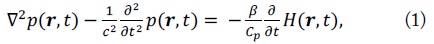
In thermoacoustic, in response to a heat source H(r,t) and without considering thermal diffusion and kinematical viscosity, the pressure p(r,t) at position r and time t in an acoustically homogenous liquid-like medium obeys the following wave equation [11,12]:

where p(r,t) is the thermoacoustic pressure at the position r and time t, c is the speed of sound, β is the isobaric volume expansion coefficient, C_p is the heat capacity, and H(r,t) is the heating function defined as the thermal energy deposited by the electromagnetic radiation per unit time and per unit volume.

In general, the solution to Eq. (1) in the time domain can be expressed by [9]

H(r,t) can also be described by a specific absorption rate (SAR). The SAR is usually adopted as a standard of energy absorption rate when tissue is exposed to radio frequency radiation and is defined as [7],

where |E| is the amplitude of the electric field intensity, σ is the conductivity, ρ is the mass density, I(t) is the envelope of the instantaneous power of the microwave signal, t is the time, and r is the spatial location of a point on the object.

To obtain the heating function data, we need the electric field data at position r and time t, as shown in Eq. (3). Therefore, a simulation is conducted using CST Microwave Studio to obtain the data of the electric field absorbed by the object.

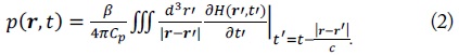
The thermoacoustic simulation model is shown in Fig. 1. The object is a fat (ε_r=5.44) cylinder with a diameter of 50 mm and a height of 20 mm. This cylinder receives electromagnetic radiation from an antenna placed 10 mm under the bottom surface of the cylinder. The antenna used in this simulation is a dipole antenna λ/2.

Both the cylinder and the antenna are surrounded by oil (ε_r=2.1) as a coupling medium. In the real thermoacoustic experiment, the mechanical wave requires a coupling medium to propagate and to be detected by the transducer.

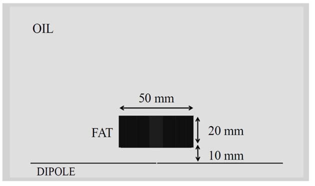
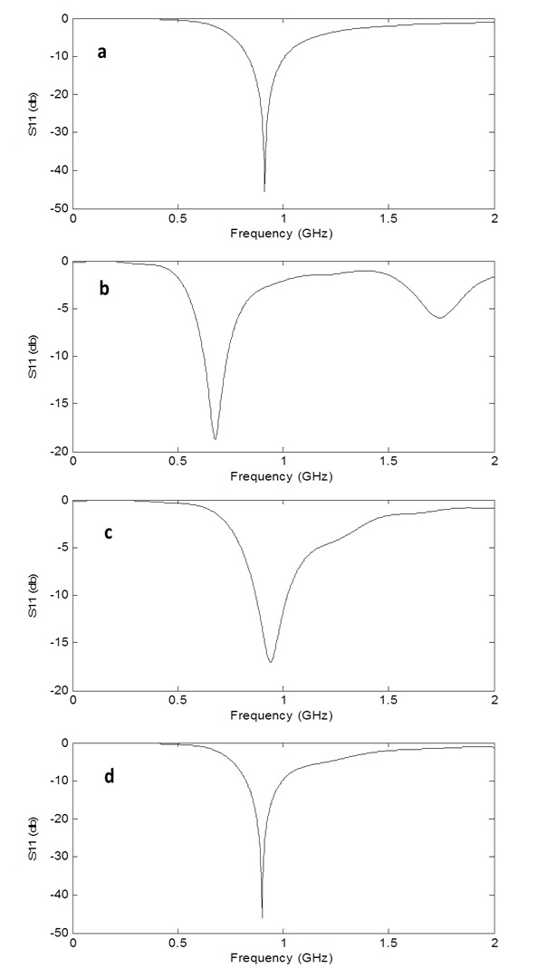
Fig. 2(a) shows the reflection coefficient for the dipole antenna that works at a frequency of 0.9 GHz. To obtain a good reflection coefficient, the impedance at the antenna port is matched with the antenna’s radiation impedance. For the dipole antenna, the radiation impedance is 168 Ω [13]. In Fig. 2(b), the same antenna as in Fig. 2(a) is simulated in oil as coupling material.

In this case, the working frequency is shifted to 0.7 GHz. To reobtain the working frequency of 0.9 GHz, the dipole antenna length is shortened to 110 mm (previously 168 mm). The result of changing the antenna length is shown in Fig. 2(c). In Fig. 2(d), a better reflection coefficient is obtained by matching the port impedance with the antenna’s radiation impedance of 110 Ω, which is smaller than the previous value as the impedance is affected by ε_r of the coupling material this time.

The pulsed signal used to irradiate the object has a Gaussian envelope modulation. Simulation is conducted using the Gaussian pulse with a 10-MHz bandwidth. The pulse shape and its frequency spectrum are shown in Fig. 3.

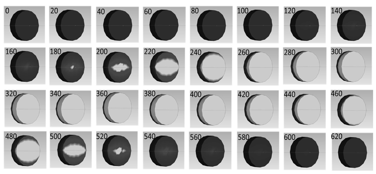
Fig. 4 shows the 3D simulation result after radiating the object with a 10-MHz bandwidth Gaussian pulse. The result shows the electric field distribution absorbed by the object. The numbers on the upper corner of each picture show the time instance in nanoseconds. The brightness shows the intensity of the E-field absorbed by the object; a dark color means a low intensity of E-field, and a light color means a high intensity of E-field. Given the E-field data at position r and time t, we can calculate the heating function that is proportional to the squared electric field value.

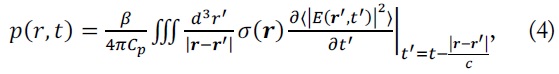
To observe the shape of the time-varying heating function data at any point on the target, a time-varying electric field at one particular point on the object is observed (the position of that particular point is marked with an x in Fig. 5, as observed from the side and top views). Fig. 5 shows that the shape of the time-varying heating function data (represented by |E|²) follows the shape of the Gaussian envelope of the radiated pulse.

Eq. (2) can also be written as [14],

where |E| is the amplitude of the electric field intensity, σ is the conductivity, r is the position of the transducer (where the thermoacoustic signal is observed), and r' is the position inside the object where microwave is absorbed and acoustic signal is generated.

The term is constant, and σ(r) is also constant for an object with a uniform material, e.g., fat only. All of the constant terms are not included in this part for the sake of simplicity. The term indicates the first time derivative of the squared electric field value at position r'. Note that in this term, t' is used instead of t. The term shows that for positions with different distances |r-r′| from the transducer, the resultant signal will have a different shift To obtain an accurate result, Eq. (4) should be handled by applying numerical integration. However, to simplify and roughly estimate the resultant pressure signal, one can do a simple summation of the generated thermoacoustic pressure in every position inside the object. This method is useful and does not need any complicated calculation.

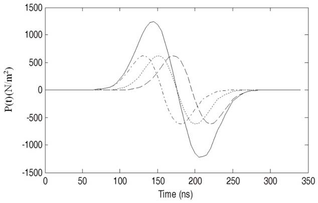
The thermoacoustic signal generated by only one point inside the object is shown in Fig. 6. The shape follows the first time derivative of the Gaussian envelope. Fig. 7 shows an example to describe the summation of the thermoacoustic signals from three points inside the object with different shifts (i.e., different distances to the transducer). The total signal after summation is represented by the solid line.

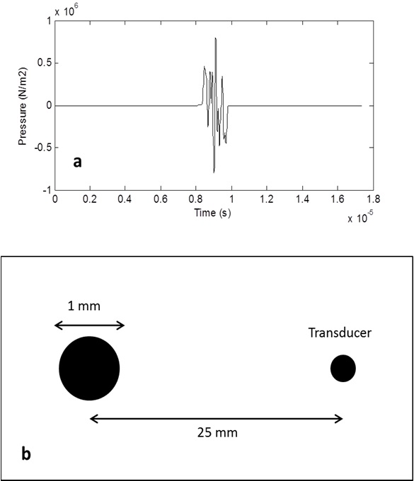
Another simulation is conducted using the same setting with previous heating function simulations, but this time the irradiated object is a small sphere with a 1 mm diameter. The point transducer is assumed to be placed 25 mm from the object.

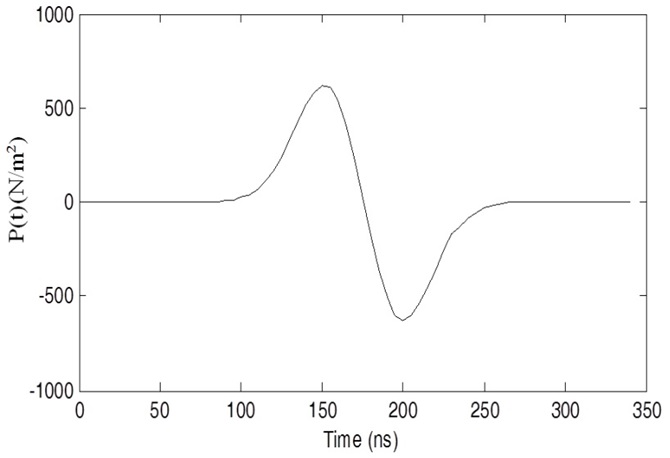
The generated thermoacoustic signal from the fat sphere object, observed from a point transducer placed 25 mm from the object, is shown in Fig. 8. The shape shows two peaks, one positive peak and one negative peak, corresponding with the shape of the first time derivative of the Gaussian envelope.

Computer simulations are conducted to obtain absorbed electric field data. Heating function data are then calculated using the provided electric field data. The thermoacoustic signal received at a point transducer with a specified distance from the object is calculated by incorporating the heating function data into a thermoacoustic equation. The integration part is simplified by performing a summation of the individual thermoacoustic signals from all points inside the object.

The shape of the time-varying heating function data follows the envelope of a Gaussian pulse used in excitation. The shape of the thermoacoustic signal follows the first time derivative of the Gaussian pulse envelope.

The simulations conducted provide the simplest explanation to the thermoacoustic phenomenon applied on thermoacoustic systems. Understanding the basic concept of thermoacoustic is the first step to implement it into more complex simulations and real experiments.

Future research to be developed will be related to the application of the thermoacoustic phenomenon to imaging, including the comparison between thermoacoustic imaging and other imaging methods such as ultrasound and conventional microwave imaging. In future experiments, the specification and sensitivity of the transducer will be provided to prove the feasibility of applying this approach to imaging.