When financial markets are unconstrained, redundant (financial) assets do not play a role in risk-sharing and thus they are useless. Therefore, without loss of generality, we can assume that there is no redundant asset. In reality, however, redundant assets such as futures and options exist because financial markets are subject to portfolio constraints. In financial markets, agents usually face portfolio constraints when they trade financial assets. Portfolio constraints capture market frictions such as short-selling constraints, credit limits, bid-ask spreads, margin requirements, and proportional transaction costs. It is noted that many of portfolio constraints (e.g., margin requirements) depend on asset prices. It is important to investigate how redundant assets and endogenous portfolio constraints affect equilibrium asset prices in financial markets.

The purpose of this paper is to show that there exists a competitive equilibrium in an exchange economy with incomplete financial markets, where agents are subject to portfolio constraints depending on asset prices. Aouani and Cornet (2011) and Hahn and Won (2014) among others demonstrate the existence of a competitive general equilibrium in an exchange economy with incomplete markets, where each agent’s asset trading is subject to exogenous portfolio constraints, which do not depend on endogenous variables. However, when agents participate in financial markets, they are often faced with endogenous portfolio constraints such as margin requirements, which depend on asset prices.

Several recent papers have studied this problem, including Carosi et al. (2009) and Cea-Echenique and Torres-Martinez (2014), among others. Carosi et al. (2009) describe portfolio constraints by restriction functions, which depend on first-period consumption and commodity prices, as well as financial asset prices. They assume that portfolio restriction functions are continuously differentible in order to characterize the generic regularity of equilibrium. Thus such approach cannot cover cases in which portfolio constraints are represented by convex cones (e.g., margin requirements). Moreover, by assuming that the payoff matrix has a column full rank, they exclude redundant assets such as financial derivatives, whose raison d'être is portfolio constraints.

Cea-Echenique and Torres-Martinez (2014) employ endogenous trading constraints represented by correspondences that depend on both commodity and asset prices. Restrictions on consumption and portfolio choices are incorporated into a single trading constraint set. Trading constraints are so general and can therefore cover collateralized borrowing constraints and income-based portfolio constraints. In particular, attainable allocations are price-dependent. However, they impose a restrictive assumption that the set of price-dependent attainable allocations is bounded. This assumption may not be fulfilled in constrained incomplete markets with redundant assets, in which asset demand correspondences are unbounded. Therefore, they de facto exclude financial derivatives from incomplete financial markets.

The rest of the paper is organized as follows: in Section II, we present the model of an exchange economy with incomplete markets where each agent is faced with endogenous portfolio constraints. In Section III, we define constrained arbitrage and provide additional assumptions for endogenous portfolio constraints. Section IV contains examples of endogenous portfolio constraints. In Section V, we show that a competitive equilibrium exists in the economy and present a numerical example of a competitive equilibrium. Section VI contains the concluding remarks.

The paper considers an exchange economy with financial asset markets, extending over two periods. There are I agents and J financial assets. The uncertainty of the second period is described by a finite set S :＝{1, ..., S} of states of nature. In the first period, no agent knows which state will be realized in the second period. The payoffs of asset j∈J :＝{1, 2, ..., J } are realized depending on the state in the second period. There are L commodities in each state s＝S₀ :＝S◡{0} where the first period is regarded as state s＝0. Therefore, the commodity space is equal to Rℓ where ℓ:＝L(S＋1).

In the first period, agent i∈I :＝{1, 2, ..., I} makes consumption x_i(0) and invests portfolio θ_i with his endowments. In the second period, agent i makes consumptions (x_i(s))_s∈S with his endowments and payoffs of his portfolio. Hence, agent i chooses consumption bundle x_i:＝(x_i(0), x_i(1), ..., x_i(S)) in his consumption set X_i⊂R^ℓ, which contains his initial endowment e_i of commodities. Preferences over X_i are represented by a preference relation ≻i on X_i, which is irreflexive, complete, and transitive. The preference relation ≻i defines the preference correspondence P_i:X_i →. by P_i(x_i) :＝{ ∈X_i :≻_ix_i}, which is the set of consumption bundles that agent i prefers to x_i. Agent i is subject to portfolio constraints, as represented by correspondence Θ_i : R^J → 2^RJ of asset price q∈R^J. To finance his consumption in the second period, agent i chooses portfolio θ_i∈Θ_i(q) in the first period.

The payoff of asset j in state s∈S is denoted by r_j(s), and the payoff vector of asset j over S states by an S dimensional column vector r_j＝(r_j(s))_s∈S. Payoff vector in state s is denoted by a J dimensional row vector r(s)＝(r_j(s))_j∈J. We denote the asset payoffs by an (S×J) payoff matrix R＝[(r_j)_j∈J]. An asset is called redundant if its payoffs can be replicated by those of the other assets. We allow redundant assets, i.e., V^⊥≠{0} where V^⊥＝{θ ∈R^J: R⋅θ ＝0}. We note that redundant assets do not play a risk-sharing role without portfolio constraints because their payoffs can be replicated by those of the other assets. In contrast, redundant assets participate in risk-sharing under portfolio constraints, which may prevent the replication of redundant assets. We represent this economy by E＝<(X_i, ≻_i, e_i, Θ_i)_i∈I; R>.

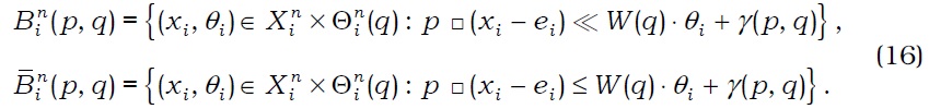
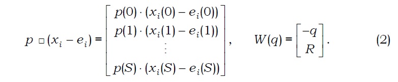
In the first period, agent i is subject to budget constraint p(0)⋅x_i(0)＋q⋅θ_i≤p(0)⋅e_i(0), where (p(0), q)∈R^L×R^J is a vector of commodity and asset prices in the first period. In the second period, he is subject to budget constraint p(s)⋅x_i(s)≤p(s)⋅e_i(s)＋r(s)⋅θ_i, ∀s∈S, where p(s)∈R^L is a vector of commodity prices at state s∈S. Therefore, given price vector (p, q)∈R^ℓ× R^J, agent i maximizes his preference ≻i by choosing a pair (x_i, θ_i) of consumption and portfolio in his budget set:1

where

A pair (x_i, θ_i)∈B̅_i(p, q) is optimal for agent i if [P_i(x_i)×Θ_i(q)]⌒B̅_i(p, q)＝∅.

Definition 2.1: A competitive equilibrium of economy E is a profile (p^*, q^*, x^*, θ^*)∈R^ℓ×R^J×(R^ℓ)×(R^J)^I, such that

We now provide the list of basic assumptions for every agent i∈I, which are necessary for our main results.

Note that Assumptions (A1)-(A5) are standard assumptions. Assumption (A6) states that the portfolio constraint of agent i is represented by a convex-valued correspondence that has a closed graph. Moreover, Assumption A6 requires that portfolio constraints ‘nicely’ depend on asset prices. This assumption can cover market frictions such as short-selling constraints, bid-ask spreads, margin requirements, and proportional transaction costs.8 Moreover, Assumption (A6) states that portfolio choice sets depend solely on the relative price of assets.

1Let v and v’ be vectors in a Euclidean space. Then v≥v’ implies that v－v’∈ Rℓ＋; v＞v’ implies that v≥v’ and v≠v’; and v≫v’ implies that v－v’∈Rℓ＋＋.  2Note that B̅i is a correspondence from Rℓ×RJ to Rℓ×RJ.  3The preference relation ≻i is continuous if Pi(xi) and Pi－1(xi) :＝{xi’∈Xi : xi≻ixi’} are open for every xi∈Xi, and is convex if Pi(xi) is convex for every xi∈Xi.  4For each xi∈Xi and for each s∈S there exists xi’(s)∈Xi(s) such that (xi’(s), xi(－s))≻ixi, where xi(−s) = (xi(0),…, xi(s − 1), xi(s + 1),…, xi(S)).  5Let A be a non-empty subset of a Euclidean space. The closure of A is denoted by cl(A) and the interior of A is denoted by int(A).  6Let X and Y be subsets of Euclidean space. A correspondence ϕ : X→2Y is lower hemicontinuous if {x∈X: ϕ(x)⌒V≠∅} is open for every open set V⊂Y and has a closed graph if Gϕ:＝{(x, y)∈X×Y: y∈ϕ(x)} is closed.  7The homogeneity of degree zero for constrained choice sets can be also found in and Page and Wooders (1999) and et al Carosi et al. (2009).  8See Heath and Jarrow (1987), Luttmer (1996), and Elsinger and Summer (2001).

When no portfolio constraints are present in incomplete markets, no arbitrage opportunity is admitted and therefore the law of one price holds in equilibrium. However, the law of one price does not hold in incomplete markets with portfolio constraints, and it is not appropriate to apply the notion of arbitrage used for unconstrained incomplete markets to constrained incomplete markets. The notion of constrained arbitrage is employed in Jouini and Kallal (1999) and Luttmer (1996), which study incomplete markets with exogenous portfolio constraints. To introduce an appropriate notion of arbitrage for incomplete markets with endogenous portfolio constraints, let C_i(q) denote the recession cone Γ(Θ_i(q)) of Θ_i(q).9

Definition 3.1: Asset price q∈R^J is said to admit a constrained arbitrage for agent i if there is a portfolio θ_i∈C_i(q), such that W(q)⋅θ_i＞0. Asset price q∈R^J is said to admit no constrained arbitrage for economy E if it admits no constrained arbitrage for every agent i∈I.

No constrained arbitrage is equivalent to no arbitrage in unconstrained incomplete markets. Let Q_i denote the set of asset prices that admit no constrained arbitrage for agent i. Then, Q: ∩_i∈IQ_i is the set of asset prices that admit no constrained arbitrage for E. Let N_i(q) be the lineality space of Θ_i(q).10 We define N₀(q)＝Σ_i∈I(N_i(q)⌒V^⊥) and denote by N₀(q)^⊥ its orthogonal complement in R^J. Let us define Q^*:＝{q∈Q: q∈N₀(q)^⊥}. The following results show what is appropriate for equilibrium asset prices.

Proposition 3.1: It holds that Q and Q^* are non-empty.

Proof : To show Q≠∅, suppose otherwise, that is, Q＝∅. Consider q＝λ ⋅R with λ ∈. Since Q＝∅, we see that q∉Q. Then there is some agent i with θ_i∈C_i(q) satisfying W(q)⋅θ_i＞0, which makes q⋅θ_i＝λ⋅R⋅θ_i≥0 necessary. If q⋅θ_i＞0, then q∈Q, then q∈Q, which is a contradiction. If q⋅θ_i＝λ ⋅R⋅θ_i＝0, then R⋅θ_i＝0. This implies that q∈Q, which is a contradiction. Hence, Q is non-empty.

To show Q^*≠∅, suppose otherwise, that is, Q^*＝∅. Take any q∈Q, and we have q∉N₀(q)^⊥. Then there exists v∈N₀(q) such that q⋅v＜0 without loss of generality. Since there exists v_i∈N_i(q)⌒V^⊥, ∀i∈I such that v＝Σ_i∈Iv_i, it follow that q⋅v_i＜0 for some i. Noting that v_i∈C_i(q) and R⋅vi＝0, we see that v_i is a constrained arbitrage opportunity at q. Therefore, q∉Q_i and q∉Q, which is a contradiction. Hence, Q^* is nonempty.

Proposition 3.2: Under Assumption (A4), an equilibrium asset price q belongs to Q^*.

Proof: Let (p, q, x, θ) be an equilibrium of E. Suppose that q∈Q. Then there is some i∈I with v_i∈C_i(q) satisfying W(q)⋅v_i＞0. This implies that θ_i＋v_i∈Θ_i(q) and W(q)⋅θ_iW(q)⋅(θ_i＋v_i). Due to Assumption (A4), there exists a consumption bundle x_i’∈X_i, such that x_i’≻_ix_i and (x_i’, θ_i＋v_i)∈B̅_i(p, q), which contradicts the optimality of (x_i, θ_i ) in B̅_i(p>, q). Hence, q∈Q.

We now show that q∈N₀(q)^⊥, that is, q⋅v＝0 for all v∈N₀(q). Suppose otherwise. Then there exists v∈N₀(q) such that q⋅v<0 without loss of generality. Since there exists v_i∈N_i(q)⌒V^⊥, ∀i∈I such that v＝Σ_i∈I v_i, it follow that q⋅v_i＜0 for some i. Noting that v_i∈C_i(q) and R⋅v_i＝0, we see that v_i is a constrained arbitrage opportunity at q. That is, q∉Q_i, and therefore q∉Q, which is a contradiction. Hence, q∈N₀(q)^⊥. ■

From Proposition 3.2, we see that Q^* is an appropriate set of equilibrium asset prices and that Q and Q^* appear as cones with vertex zero under Assumption (A6). We observe that Q^* may not be convex. Therefore we consider Q̂ which is the convex hull of Q^*. Then Q̂ is a nonempty convex cone.

We now impose a portfolio survival condition, which states that there is no constraint on trading for sufficiently small amount of portfolios.

To analyze the effects of redundant assets on risk-sharing in constrained asset markets, we need to examine feasible zero-income portfolios. We call portfolios in C_i(q)⌒V^⊥ scale-free feasible zero-income portfolios for agent i in that, if v_i∈C_i(q)⌒V^⊥, we have λ v_i∈Θ_i(q) and R⋅(λv_i)＝0 for every λ≥0. Particularly, if q∈cl(Q̂)\{0}, some agent i may have a portfolio v_i∈C_i(q)⌒V^⊥ satisfying q⋅v_i≤0. Therefore, in the presence of scale-free feasible zero-income portfolios, some agent’s portfolio choices may be unbounded with his budget constraint satisfied. To prevent such negative effect of scale-free feasible zero-income portfolios at the aggregate level, we need the following assumption:

If Assumption (A8) does not hold, there is an asset price q∈cl(Q̂)\{0}, such that some agent i has a scale-free feasible zero-income portfolio v_i∈C_i(q)⌒V^⊥, which is supported by the other agents because －v_i∈Σ_j≠iC_j(q)⌒V^⊥. Therefore, agent i can hold an indefinite amount of portfolios in the direction of v_i such that the budget constraints of all agents and the market clearing condition are not violated. This possibility is eliminated by Assumption (A8).

9Let A be a non-empty convex subset of Euclidean space X. The recession cone of A is the set Γ(A)＝{v∈E: A＋v⊂A}. When A is closed, Γ(A) is also closed and can be expressed as Γ(A)={v∈X:∃{xn} in A and {an} in R. with an → 0 such that anxn → v}  10The lineality space L(A) is the maximal subspace in A, that is, L(A)＝Γ(A)⌒[－Γ(A)].

Financial intermediaries prohibit short-selling above specific limits, which can depend on asset prices. Financial regulation prohibits the purchase of some securities above given limits, which may also depend on asset prices. Let continuous functions a_i: R^J→R^J and b_i: R^J→R^J take the values of the short-selling limits or buying limits of agent i on securities, respectively. The portfolio constraints of agent i can therefore be described by

where 0∈(a_i(q), b_i(q)), ∀q∈R^J, a_i: R^J→R^J, and b_i: R^J→R^J are continuous functions and homogeneous of degree zero in q.

Financial intermediaries can provide credit to agents with limits that depend on asset prices. In this case, the trading strategies of agent i are restricted such that

where a_i: R^J→R_＋＋ is a continuous function and homogeneous of degree one in q and b_i: R^J→ is a continuous function and homogenous of degree zero in q.

Financial assets such as collateralized debt obligation (CDO) are used as debt instruments and should be backed by a pool of other financial assets. Supposing that security 1 is a risk-less bond, we can express portfolio constraints in the following form:11

where θ_i^－＝(－min{0, θ_ij})^J_j＝1, θ_i^＋＝(max{0, θ_ij})^J_j＝1, a_i∈R_＋, and b_i∈R_＋＋. It is obvious that the portfolio correspondences of the above examples satisfy Assumptions (A6) and (A7).

As in Heath and Jarrow (1987), portfolio constraints that involve margin requirements can be described as

where security 1 is risk-less bond, a_i≥2, and b_i∈R_＋＋. For example, assume that J＝2 and b_i＝0.12 Suppose that security 1 is risk-less bond and security 2 is a stock. Now suppose that agent i shorts one stock and maintains a margin account with mi proportion of the stock price in the bond. The portfolio constraint is therefore reduced to

which implies that m_i≥a_i/(a_i－1). In the case where a_i＝3, we have m_i≥3/2, that is, agent i should put the money from shorting the stock and an additional fifty percent of the stock price in his margin account.

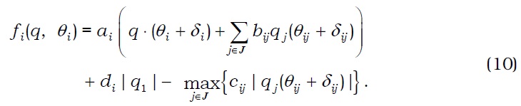
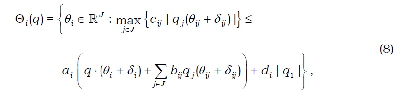
Won (2003) provides a more generalized form of the example in Heath and Jarrow (1987). Assuming that security 1 is a risk-less bond with q_i＝1, we modify his example to present the portfolio constraint set of agent i at q∈cl(Q)\{0} by

where a_i≥1, b_ij≥0, c_ij≥0, d_i＞0, and δ_ij＞0 are constants for every i and j and δ_i＝(δ_ij). It is obvious that Θ_i has a closed graph and satisfies the homogeneity of degree zero. If we assume that

we have 0∈lnt(Θ_i(q)), ∀q∈cl(Q)\{0}. To see that Θ_i is convex-valued, we define continuous function : R^J × R^J→R by

The portfolio constraint correspondence is then given by

We can observe that max_j{⋅} is a convex function on R^J and |⋅| is a convex function on R, which implies that －max_j∈J {c_ij|q_j(θ_ij＋δ_ij)|} is a concave function of θ_i. Hence, we see that is a concave function function of θ_i and therefore Θ_i is convex-valued.

To show that Θ_i is lower hemicontinuous, we define correspondence Θ_i°: R^J →2^RJ by

Suppose θ_i^*∈Θ_i°(q^*), that is, (q^*, θ_i^*)＞0. Take a sequence {(qⁿ, θ_iⁿ)} converging to (q^*, θ_i^*). Since is continuous, for sufficiently large n,

which implies that θ_iⁿ∈Θ_i°(qⁿ). Thus we see that Θ_i° is lower hemicontinuous. Noting that Θ_i(q)＝cl(Θ_i°(q)), we see that Θ_i is lower hemicontinuous. Hence, Θ_i satisfies Assumptions (A6) and (A7). □

11This example is adapted from Elsinger and Summer (2001).  12To be precise, bi should be sufficiently close to zero.

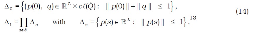
In this section, we will show that there exists a competitive equilibrium of economy E. We define the sets of normalized prices by Δ＝Δ₀×Δ₁, where

We observe that Δ is compact and convex.

̂Let X :＝Π_i∈I X_i and A_X :＝{(x₁, ..., x _I)∈X: Σ_i∈I (x_i－e _i)＝0}. We denote by X̂_i the projection of X_i onto A_X and let X̂: Π_i∈I X̂_i. To consider a sequence of truncated economies, we take an increasing sequence {(K_n, M_n)} of compact convex cube pairs with center 0 such that K_n⊂R^ℓ with X̂_i⊂int(K₁), and M_n⊂R^J with 0∈int(M₁) which satisfy ∪_nK_n＝R^ℓ and ∪_nM_n＝R^J. For each n and _i∈I, we define X_iⁿ :＝X_i⌒K_n, Θ_iⁿ(q) :＝Θ_i(q)⌒M_n, X_n :＝Π_i∈I X_iⁿ, and Θⁿ(q) :＝Π_i∈I Θ_iⁿ(q). Moreover, the preference correspondence P_iⁿ : X_iⁿ → 2X_iⁿ is defined by P_iⁿ (x_i) :＝P_i(x_i)⌒X_iⁿ.

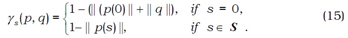
We denote by Eⁿ the truncated economy <(X_iⁿ, P_iⁿ, e_i, Θ_iⁿ)_i∈I>. We observe that each X_iⁿ is compact and each Θ_iⁿ is lower hemicontinuous with non-empty compact convex values and has a closed graph. Moreover, each P_iⁿ inherits the properties of P_i. We define function γ : Δ → R^S＋1 by γ (p, q)＝(γ_s(p, q))_s∈S0 with S₀＝S◡{0}, where

Let Ψ_iⁿ＝Mn, ∀ i∈I, and Ψⁿ＝Π_i∈I, Ψⁱ. For every i∈I and every n, we define correspondences B _iⁿ: Δ → 2X_iⁿ×Ψ_iⁿ and B̅_iⁿ: Δ → as follows:

Proposition 5.1: Under Assumptions (A1)-(A7), for each n, there is a profile (pⁿ, qⁿ, xⁿθⁿ)∈Δ×Xⁿ×Θⁿ(qⁿ) such that

where zⁿ(s):= Σ_i∈I(x_iⁿ(s)-e_i(s)) for every s∈S₀.

Proof: See Appendix. ■

Lemma 5.1: Suppose that Assumption (A6) holds. Let {(qⁿ, θ_iⁿ)} be a sequence in R^J × R^J with qⁿ → q^* and θ_iⁿ∈Θ_i (qⁿ). Suppose that {a_n} be a sequence in R_＋, such that a_n → 0. If sequence {a_n θ_iⁿ } converges to v_i, then v_i∈C>_i(q^*).

Proof: Apply 3.2 Lemma on p. 396 of Page (1987) to Θ_i. ■

From Proposition 5.1, we obtain an equilibrium existence theorem for economy E.

Theorem 5.1: Under Assumptions (A1)-(A8), economy E has a competitive equilibrium.

Proof: Take a sequence {(pⁿ, qⁿ, xⁿθⁿ)} of profiles obtained in Propostion 5.1. Since each X_i is closed and bounded from below, X̂_i is compact and so is X̂. Noting that {(pⁿ, qⁿ, xⁿ )}∈Δ×X̂, without loss of generality, we may assume that {(pⁿ, qⁿ, xⁿ )} converges to (p^*, q^*, x^*)}∈Δ×X̂.

Claim 1: Σ_i∈I(x_i^*－e_i)＝0 and Σ_i∈Iθ_i^*＝0, where (x_i^*, θ_i^*)∈X _i × Θ_i(q^*) for each i∈I.

Proof: From (d) of Proposition 5.1, it is immediate that Σ_i∈I (x_i^*－e_i)＝0. To show Σ_i∈Iθi*＝0, we claim that sequences {θ_iⁿ} for each _i∈I are bounded. Suppose otherwise. For each n, we set a_n＝(1＋Σ_i∈I ‖θ_iⁿ‖)^－1, which converges to 0. We see that anθ_iⁿ∈Θ_i(qⁿ) and sequence {a_nθ_iⁿ} for each _i∈I are bounded. Thus, without loss of generality, it converges to v_i for each _i∈I. Since Σ_i∈I a_nθ_iⁿ＝0 for all n, it holds that Σ_i∈I v_i＝0  and Σ_i∈I‖v_i‖＝1, which implies that v_i≠0 for some _i∈I.

Using Lemma 5.1, we see that v_i∈C_i(q^*). On the other hand, pⁿ(s)⋅(x_iⁿ(s)－e_i(s))≤r(s)⋅θ_iⁿ＋γ_s (pⁿ, q ⁿ) for all n and s∈S. By multiplying both sides of the inequalities by a_n and passing to the limit, we obtain R⋅v_i≥0. In view of Σ_i∈I v_i＝0, we obtain R⋅v_i＝0, that is, v_i∈V^⊥. This implies that v_i∈C_i(q^*)⌒V^⊥. Since Σ_i∈I v_i＝0, by Assumption (A8), we obtain v_i＝0 for all i∈I, which leads to a contradiction.

Therefore, {θ_iⁿ} is bounded for each i∈I. Without loss of generality, we may assume that {θ_iⁿ} converges to θ_i^*. From Assumption (A6) and (d) of Proposition 5.1, it follows that θ_i^*∈Θ_i(q^*) and Σ_i∈Iθ_i^*＝0. □

Claim 2: γ (p^*, q^*) = 0.

Proof: This immediately follows from (e) of Proposition 5.1. □

Claim 3: (x_i^*, θ_i^*)∈B̅_i(p^*, q^*)

Proof: This directly follows from (a) of Proposition 5.1 and Claims 1 and 2. □

Claim 4: p^*(0) ≠ 0.

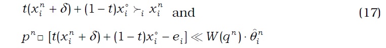
Proof: If p^*(0)＝0, agent i has x_i∈X_isuch that x_i≻_ix_i^* and (x_i, θ_i^*)∈B̅_i(p^*, q^*) in view of Assumption (A4) and Claim 3. Since p^*(s)≠0, ∀s∈S due to Claim 2, by Assumption (A5), there is x_i°∈int(X_i) such that p^*(s)⋅x_i°(s)≪p^*(s)⋅e_i(s), ∀s∈S. Since ‖q^*‖＝1 by Claim 2, Assumption (A7) ensures that there exists θ_i°∈int(Θ_i(q^*)) such that q^*⋅θ_i°＜0. Then, for t∈(0, 1) sufficiently close to 1, we see that tx_i＋(1－t) x_i°≻_ix_i^* and p^*□ [tx_i＋(1－t)x_i°－e_i]≪W(q^*)⋅[tθ_i^*＋(1－t) θ_i°] with tθ_i^*＋(1－t) θ_i°∈Θ_i(q^*). Since Θ_i is lower hemicontinuous, there exists a sequence {θ̂_iⁿ} converging to t(θ_i^*＋(1－t) θ_i° such that θ̂_iⁿ∈Θ_i(qⁿ), ∀n. Therefore, for sufficiently large n, we have tx_i＋(1－t) x_i°≻_ix_iⁿ and pⁿ□ [tx_i＋(1－t)x_i°－e_i] ≪W(qⁿ)⋅θ̂_iⁿ with tx_i＋(1－t)x_i°∈X_iⁿ and θ̂_iⁿ∈Θ_iⁿ(qⁿ). This is a contradiction in view of of Proposition (b) and (e) of Proposition 5.1. Hence, it follows that p^*(0)≠0. □

Claim 5: q^*∈Q^*.

Proof: First, we show that q^*∈Q. Suppose otherwise. Then there is some agent i who has a portfolio θ_i ∈C_i(q^*) satisfying W(q^*)⋅θ_i＞0. Assumption (A4) ensures that there exists δ∈R^ℓ such that x_i^*＋δ≻_ix_i^* and p^*□δ＜W(q^*)⋅θ_i. Claim 3 implies that p^*□(x_i^*＋δ－e_i)＜W(q^*)⋅( θ_i*＋θ_i) with θ_i*＋θ_i∈Θ_i(q^*). Note that Claims 2 and 4 imply that p*(s)≠0, ∀s∈S₀. Assumption (A5) allows us to take x_i°∈int(Xi), such that p^*□ x_i°≪p^*□e_i. Therefore, for t∈(0, 1) sufficiently close to 1, we obtain t(x_i^*＋δ)＋(1－t)x_i°≻_ix_i^* and p^*□[t(x_i^*＋δ )＋(1－t)x_i°－e_i]≪W(q^*)⋅[t(θ_i*＋θ_i)]. Since t(θ_i*＋θ_i)∈Θ_i(q^*) and Θ_i is lower hemicontinuous, there exists a sequence {θ̂_iⁿ}converging to t(θ_i*＋θ_i) with θ̂_iⁿ∈Θ_i(qⁿ). For sufficiently large n,

with t(x_iⁿ＋δ)＋(1－t)x_i°∈X_iⁿ and θ̂_iⁿ∈Θ_iⁿ(qⁿ). This is a contradiction in view of (b) and (e) of Proposition 5.1. Hence, q^*∈Q.

We now show that q∈N₀(q^*)^⊥, that is, q^*⋅v＝0 for all v∈N₀(q^*). Suppose otherwise. Then we have some v∈N₀(q^*) such that q^*⋅v＜0 without loss of generality. Since there exists v_i∈N_i(q^*)⌒V^⊥, ∀i∈I such that v∈Σi∈Iv_i, it follow that q^*⋅v_i＜0 for some i. Noting that v_i∈C_i(q^*) and R⋅v_i＝0, we know that v_i is a constrained arbitrage opportunity at q^*. Applying the same arguments presented in the previous paragraph, we arrive at a contradiction. Hence, q^*∈N₀(q^*)^⊥ and therefore q^*∈Q⌒N₀(q^*)^⊥, that is, q^*∈Q^*. □

Let us now define the open budget set of agent i by

Claim 6: [P_i(x_i^*)×Θ_i(q^*)]∩B_i(p^*, q^*) = ∅.

Proof: Suppose that the claim does not hold. Then there is some i∈I with (x̂_i, θ̂_i)∈ [P_i(x_i^*)×Θ_i(q^*)]⌒B_i(p^*, q^*). Noting that P_i^－1 is open-valued by Assumption (A3), we see that P_i^－1 is lower hemicontinuous. Since P_i and Θ_i are lower hemicontinuous and B_i has an open graph, the correspondence (p, q, x_i) ↦ [P_i(x_i)×Θ_i(q)]⌒B_i(p, q) is lower hemicontinuous. Therefore there is a sequence {(x̂_iⁿ, θ̂_i ⁿ)} converging to (x̂_i, θ̂_i) such that (x̂_iⁿ, θ̂_iⁿ )∈[P_i(x_iⁿ)×Θ_i(qⁿ)]⌒B_i(pⁿ, qⁿ). For each t∈(0, 1) and each n∈N, we set y_iⁿ(t) :＝(tx̂_iⁿ＋(1－t)x_iⁿ, tθ̂_iⁿ ＋(1－t) θ_iⁿ). Observe that, for sufficiently large n, we obtain y_iⁿ(t)∈x_iⁿ × Θ_iⁿ(qⁿ) and thus y_iⁿ(t)∈B_iⁿ(pⁿ, qⁿ) by aim 2. Therefore, for sufficiently large n, we have y_iⁿ(t)∈[P_iⁿ(x_iⁿ)×Θ_iⁿ(qⁿ)]⌒B_iⁿ(pⁿ, qⁿ), which contradicts (b) of Proposition 5.1. Hence, [P_i(x_i^*)×Θ_i(q^*)]⌒B_i(p^*, q^*)＝∅. □

Claim 7: For every i∈I, [P_i(x_i^*)×Θ_i(q^*)]∩B̅_i(p^*, q^*) = ∅.

Proof: Suppose that the claim does not hold. Then there is some i∈I with (x _i, θ_i)∈[P_i(x_i^*)×Θ_i(q^*)]⌒B̅_i(p^*, q^*). Since Claims 2 and 4 imply that p^*(s)≠0, ∀s∈S₀, by Assumption (A5), we can take (x _i’, θ_i’)∈B_i(p^*, q^*)≠∅. Assumption (A3) implies that for t∈(0, 1) sufficiently close to 1, t(x _i, θ_i)＋(1－t)(x _i’, θ_i’)∈[P_i(x_i^*)×Θ_i(q^*)]⌒B_i(p^*, q^*), which contradicts Claim 6. Hence, [P_i(x_i^*)×Θ_i(q^*)]⌒B̅_i(p^*, q^*)＝∅. □

By Claims 1, 3, and 7, we prove that (p^*, q^*, x^*, θ^*) is a competitive equilibrium for economy E. ■

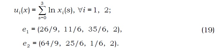
Example 5.1: We consider an exchange economy with I＝2, L＝1, J＝3, and S＝3. The utility functions and initial endowments of agents are provided as follows:

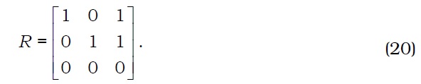
Let X_t＝R⁴_＋, ∀i＝1, 2 and consider the commodity as a numéraire. Payoff matrix is given by

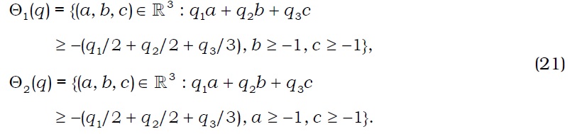
This allows us to restrict no-arbitrage asset prices to R³_＋＋. Note that V^⊥＝{v∈R³: v＝λ(1, 1, －1),λ∈R}. Portfolio constraints for agents are described by:

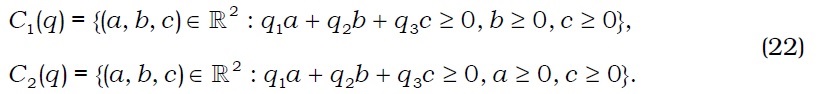
The recession cones of these constraints are:

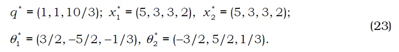
Define R_＋ :＝{θ∈R³: R⋅θ＞0}. Since C_i(q)⌒R_＋＝R³＋ for all i and q∈R³_＋＋, we find that Q＝R³_＋＋, which is a nonempty open convex cone. We denote a competitive equilibrium of the economy by (q^*, (x₁^*, x₂^*), (θ₁^*, θ₃^*))∈R²＋×(R⁴)² × (R³)². Then it follows that

Since C_i(q^*)⌒V^⊥＝{0} for all i＝1, 2, we see that Assumption (A8) is trivially holds. Note that the law of one price does not hold and that thefirst inequality constraint of agent 1 is binding at the equilibrium. □

13‖⋅‖ is the Euclidean norm.

It is shown that there exists a competitive equilibrium in a two-period exchange economy with incomplete markets where redundant assets are present and portfolio constraints are represented by a lower hemicontinuous correspondence of asset prices. Most of general equilibrium models, which study incomplete markets with endogenous portfolio constraints, either express portfolio constraints in terms of differentiable restriction functions that describe the boundary of constraints, or de facto exclude redundant assets. The present paper not only models endogenous portfolio constraints via correspondences of asset prices, but also considers the risk-sharing role of redundant assets in incomplete markets. Assumption (A8) plays a key role of excluding the unboundedness of scale-free zero-income portfolios, which arises due to redundant assets. Future possible directions of research include weakening Assumption (A8) for more general results and extending the results of this paper to economies with multiperiod incomplete markets.