Multiprecision multiplication is the most expensive operation in public key-based cryptography. Therefore, many multiplication methods have been studied intensively for several decades. In Workshop on Cryptographic Hardware and Embedded Systems 2011 (CHES2011), a novel multiplication method called ‘operand caching’ was proposed. This method reduces the number of required load instructions by caching the operands. However, it does not provide full operand caching when changing the row of partial products. To overcome this problem, a novel method, that is, ‘consecutive operand caching’ was proposed in Workshop on Information Security Applications 2012 (WISA2012). It divides a multiplication structure into partial products and reconstructs them to share common operands between previous and next partial products. However, there is still room for improvement; therefore, we propose a finely designed operand-caching mode to minimize useless memory accesses when the first row is changed. Finally, we reduce the number of memory access instructions and boost the speed of the overall multiprecision multiplication for public key cryptography.
Public key cryptography methods such as RSA [1], elliptic curve cryptography (ECC) [2], and pairing [3] involve computation-intensive arithmetic operations; in particular, multiplication accounts for most of the execution time of microprocessors. Several technologies have been proposed to reduce the execution time and computation cost of multiplication operations by decreasing the number of memory accesses, i.e., the number of clock cycles.
A row-wise method called ‘operand scanning’ is used for short looped programs. This method loads all operands in a row. The alternative ‘Comba’ is a common schoolbook method that is also known as ‘product scanning.’ This method computes all partial products in a column [4]. ‘Hybrid scanning’ combines the useful features of ‘operand scanning’ and ‘product scanning.’ By adjusting the row and column widths, we can reduce the number of operand accesses and result updates. This method has an advantage over a microprocessor equipped with many general-purpose registers [5]. ‘Operand caching,’ which was proposed recently in [6], significantly reduces the number of load operations, which are regarded as expensive operations, via the caching of operands. However, this method does not provide full operand caching when changing the row of partial products. Recently, a novel method caches the required operands from the initial partial products to the final partial products. However, there is still room for further improvement in performance.
In this paper, we propose a novel efficient memory access design to minimize the number of operands and intermediate results accesses when the first row is changed. Finally, the number of required load/store instructions is reduced by 5.8%.
The remainder of this paper is organized as follows: In Section II, we describe different multiprecision multiplication techniques, and in Section III, we revisit the operandcaching method and then, present the optimal memory access method. In Section IV, we describe the performance evaluation in terms of memory accesses and clock cycles. Finally, Section V concludes the paper.
II. MULTIPRECISION MULTIPLICATION AND SQUARING
In this section, we introduce various multiprecision multiplication techniques, including ‘operand scanning,’ ‘product scanning,’ ‘hybrid scanning,’ and ‘operand caching.’ Each method has unique features for reducing the number of load and store instructions. In particular, ‘operand caching’ reduces the number of memory accesses by caching operands to the registers. However, after the calculation of partial row products, no common operands exist. Therefore, operands should be reloaded for the next row computation. To overcome this problem, we present an advanced operand-caching method that ensures operand caching throughout the processes. As a result, the number of required load instructions decreases.
To describe the multiprecision multiplication method, we use the following notations: let A and B be two
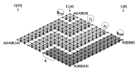
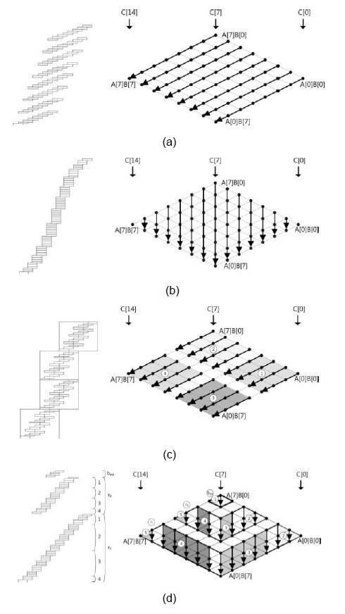
For the sake of clarity, we describe the method by using a multiplication structure and a rhombus form, as shown in Fig. 1. Each point represents a multiplication A[
This method consists of two parts, i.e., inner and outer loops. In the inner loop, operand A[
Fig. 1(a) shows the multiprecision multiplication technique, which is called ‘operand scanning.’ The arrows indicate the order of computation, and the computations are performed from the rightmost corner to the leftmost corner. In each row, load instructions are executed 2
This method computes all partial products in the same column by using multiplication and addition [4]. Because each partial product in the column is computed and then accumulated, registers are not needed for intermediate results. The results are stored once, and the stored results are not reloaded because all computations have already been completed. To perform multiplication, three registers for accumulation and two registers for the multiplicand, i.e., a total of five registers, are required. When the number of registers increases to more than five, the remaining registers can be used for caching operands.
Fig. 1(b) shows the multiprecision multiplication technique, which is called ‘product scanning.’ The arrows direct from the top of the rhombus to the bottom, which means that the partial products are computed in the same column. The partial products are computed from right to left. For computation, load instructions are executed 2
This method combines the useful features of ‘operand scanning’ and ‘product scanning’ [5]. Multiplication is performed on a block scale by using ‘product scanning.’ The number of rows within the block is defined as
Fig. 1(c) shows the multiprecision multiplication technique, which is called the ‘hybrid’ method, for the case of
This method follows ‘product scanning,’ but it divides the calculation into several row sections [6]. By reordering the sequence of the inner and outer row sections, the previously loaded operands in the working registers are reused for computing the next partial products. A few store instructions are added, but the number of required load instructions is reduced. The number of row sections is given by , and e denotes the number of words used to cache a digit in the operand.
Fig. 1(d) shows the multiprecision multiplication technique, which is called ‘operand caching’ in the case of
III. CONSECUTIVE OPERAND-CACHING METHOD
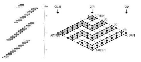
In this section, we introduce consecutive operand-caching multiprecision multiplication [7]. Because this method is based on ‘operand caching,’ it can perform multiplication with a reduced number of memory accesses for operand load instructions by using caching operands. However, the previous method has to reload operands whenever a row is changed, which generates an unnecessary overhead.
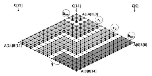
To overcome these shortcomings, the method divides the rows and re-scheduled the multiplication sequences. Thus, they found a contact point among rows that share the common operands for partial products. Therefore, they can cache the operands by sharing the operands when a row is changed. A detailed example is shown in Fig. 2.
>
A. Structure of Consecutive Operand Caching
The size of the caching operand e and the number of elements n are set to 2 and 8, respectively. The value e is determined by the number of working registers in the platform. The number of rows is
The algorithm is divided into three parts. The initialization block
The block located at the top of the rhombus executes ‘product scanning’ using operands of size (
The row parts compute the overlapping store and load instructions between the bottom and the upper rows.
The block located at the bottom of the rhombus can reuse caching operands B[0] and B[1] from
The block located between
The
>
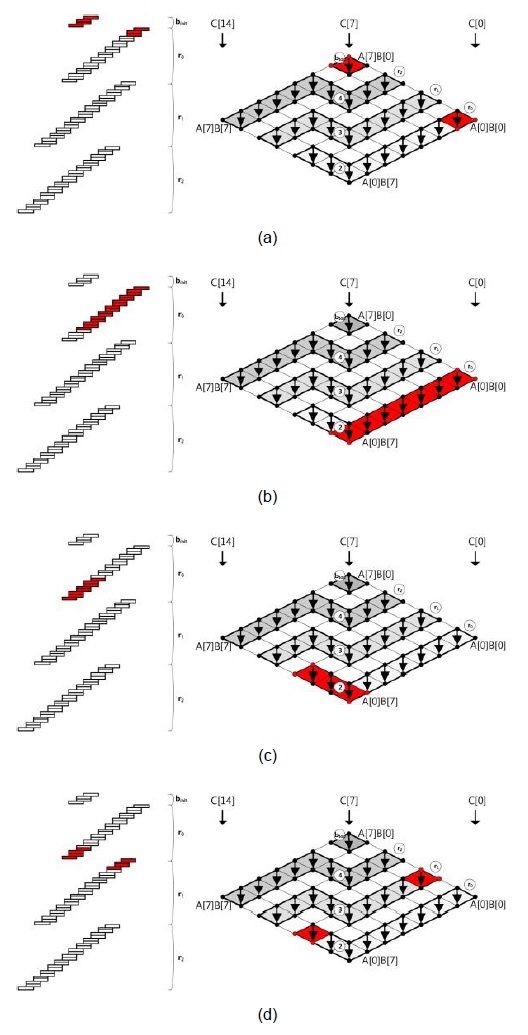
G. Consecutive Operand Caching with Common Operands
In this section, we will describe the features of common operands for consecutive operand caching. The process is computed in the following order: (a), (b), (c), and (d), as shown in Fig. 4. Firstly, in process (a),
>
H. Full Operand-Caching Multiplication
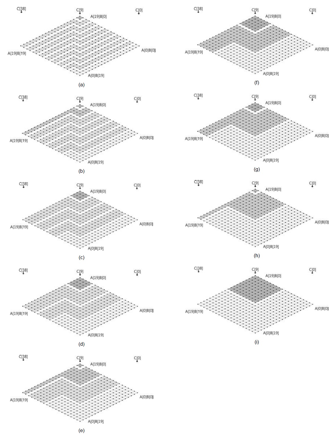
Earlier, we discussed that the operand-caching method highly optimizes the number of memory accesses by finely caching operands. However, we found that the method has room for performance improvement in the case of (
In the following section, we present two cases on the basis of the operand size (
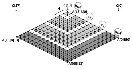
In Fig. 4, at row
- Case 1: 0 <
Case 1 is depicted in Fig. 5, where (
- Case 2: <
Case 2 is depicted in Figs. 6 and 7 where (
In this section, we analyze the complexity of memory accesses, which are expensive instructions in the practical implementations of multiprecision multiplication. To show performance enhancement, we implemented methods on a representative 8-bit AVR microprocessor.
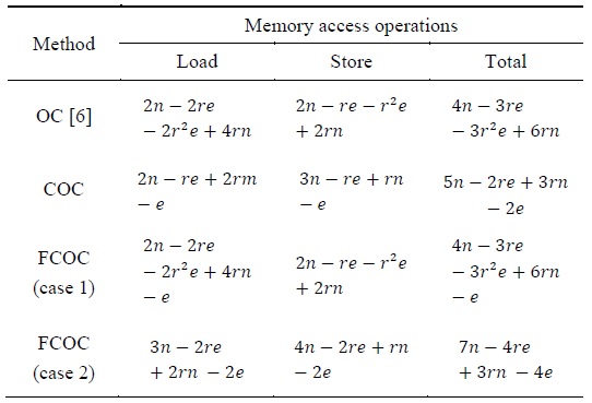
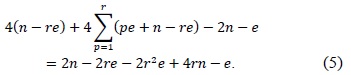
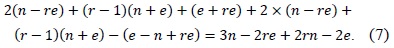
Since memory access is the most time-consuming operation, we calculated the number of memory accesses. The number of load and store instructions in the operandcaching method is calculated as follows: the notation


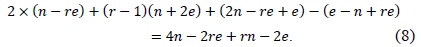
The consecutive operand-caching method is evaluated under the condition ⌊


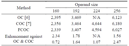
The full operand-caching method uses relatively few memory accesses including the load and store operations. In the case of normal operand caching, we can decrease the number of operand accesses by
[Table 1.] Comparison of the number of load and store instructions for multiprecision multiplication

Comparison of the number of load and store instructions for multiprecision multiplication

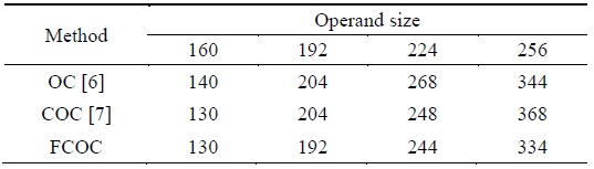
Multiprecision multiplication memory access result obtained using various methods with different operand sizes


>
B. Evaluation on 8-Bit Platform AVR
We evaluated the performance of the proposed method by using MICAz mote, which is equipped with an ATmega128 8-bit processor clocked at 7.3728 MHz. It has a 128-kB EEPROM chip and a 4-kB RAM chip [8]. The ATmega128 processor has an RISC architecture with 32 registers. Among them, six registers (r26–r31) serve as special pointers for indirect addressing. The remaining 26 registers are available for arithmetic operations. One arithmetic instruction incurs one clock cycle, and a memory instruction or memory addressing or 8-bit multiplication incurs two processing cycles. We used six registers for the operand and result pointer, two for the multiplication result, four for accumulating the intermediate result, and the remaining registers for caching operands.
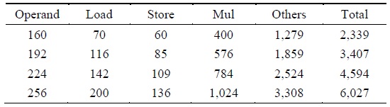
In the case of multiplication, the proposed method requires a small number of memory accesses, which can reduce the required operand access. To optimize performance, we further applied the carry-once method, which updates two intermediate results at once [9], which in turn reduces an addition operation in every intermediate update. In Table 3, we compared the proposed method including consecutive operand caching and fully consecutive operand caching with operand caching. In four representative cases, we achieved performance enhancement by 1.63% and 2.34% for consecutive operand caching and fully consecutive operand caching as compared to operand caching, respectively. The detailed instruction information is available in Table 4.
Multiprecision multiplication clock cycle result obtained using various methods with different operand size
[Table 4.] Instruction counts for the proposed multiplication on the ATmega128 (excluding PUSH/POP)

Instruction counts for the proposed multiplication on the ATmega128 (excluding PUSH/POP)
>
C. Limitation of the Proposed Method
RSA and ECC are widely used in public key cryptography. Compared to ECC, RSA requires at least 1024- or 2048-bit multiplication. The operand size is highly related to performance. When it comes to embedded processors, 2048-bit RSA is extremely slow. Recently, Liu and Großschädl [10] proposed a hybrid finely integrated product scanning method that achieved 220,596 clock cycles for 1024-bit multiplication. The problem was that the focus was only on fast implementation, and therefore, all the program codes were written in unrolled way. However, in the case of 1024-bit multiplication, the code size was about 100 kB. Furthermore, the proposed method cannot be used for all microprocessors. The MSP430 and SIMD processors have different hardware multipliers and instruction sets; therefore, a straightforward implementation of the proposed method does not guarantee high performance [9, 11]. In this case, we should carefully re-design the multiplication method to fully exploit the advantages of both specific hardware multipliers and multiplication structures.
The previous best-known method reduced the number of load instructions by using caching operands. However, there is a little room for further performance improvement, which could be brought about by reducing the number of load instructions. In this study, we attempted to achieve high performance enhancement by introducing a fully operand cached version of the previous design. The evaluation results showed an improvement in the performance of this method, brought about by an analysis of the total number of load and store instructions. For more practical results, we implemented the method using a microprocessor and evaluated the clock cycles for the operation. This algorithm could be applied to other platforms and various public key cryptography methods.

![Multiprecision multiplication techniques. (a) Operand scanning. (b) Product scanning [4]. (c) Hybrid scanning [5]. (d) Operand caching [6].](http://oak.go.kr/repository/journal/17292/E1ICAW_2015_v13n1_27_f001.jpg)
![Consecutive operand-caching method [7].](http://oak.go.kr/repository/journal/17292/E1ICAW_2015_v13n1_27_f002.jpg)