The successful operation of modern cellular mobile communication networks depends not only on initial planning, but also on adaptability to changing conditions. In large cities with developed infrastructure, the constantly changing environment requires the cellular operator to quickly react to environmental changes. Permanently increasing the volume of transmitted information requires optimization of honeycomb network configuration, the search for optimal methods for electromagnetic compatibility(EMC), and spatial frequency resource distribution for continuous monitoring of overloads. Highly effective networks operators planning, optimization, and operation of the network using expensive software using models of propagation of electromagnetic waves in various conditions, taking into account terrain based geo-information technology(GIS) and EMC control [1,2]. In the field of mobile communication network planning methods are available as frequency-territorial coverage and service areas forecasts (i.e., of coverage) for base stations (BSs).
2. Scheduling in Base Station Cellular Networks
The main task when planning mobile networks is to provide an adequate frequency plan and the necessary coverage with high quality and minimal investment in a given region. Despite the existence of well-known algorithms for constructing networks, the planning process and criteria vary depending on the relevant dominant factors and are individually selected for each task.
In general network planning is an iterative process that includes the following steps:
(1) Synthesis of the network structure; (2) Prediction of the signal field strength within the network; (3) Analysis of the service area of each cell and the entire network; (4) Assessment of the intra electromagnetic compatibility; (5) Frequency assignment; (6) Analysis of the functioning of the network, taking into account interference.
The iterative planning process continues until a radio network

The initial set of feasible options for the structure and placement of base stations, the set of performance indicators
The sequence of actions when planning a mobile network are as follows:
(1) Preparation of raw data. (2) Calibration of mathematical propagation models based on the measurements of the field strength in the most characteristic point within the network coverage. (3) Construction of a first approximation of the radio network. (4) Locating sites deploying base stations in the countryside and iterative optimization with extensive use of funds software.
The most useful approach to solving this problem is decomposition of the planning process into several stages. When this approach is applied to the problem of frequency territorial planning projects, it provides a network based on customer preferences that can be used as a reference. The main stages of frequency-spatial planning are described below.
The first stage involves preparing digital topographic maps of the area, which contain data on terrain, the development of the territory, and the locations of forests and water bodies.
The second stage consists of obtaining data regarding terrain height, land use, distributions of traffic flows, and other factors affecting signal density
Additionally, the intensity of traffic, forecasts of the number of subscribers, recommended sites for base stations, available bandwidth, compatibility with other systems, and network interfaces should be considered [3].
The third stage begins with the construction of the original radio network
In the fourth step, the binding sites deploying BSs are defined in the plan to build the network areas and perform iterative optimization of geo-information databases using special software.
In this paper, we will consider the following processes: searching sites for base stations, performing a preliminary assessment of the BS coverage areas, and calculating the technical parameters of the BS (transmitter power, suspension height, and azimuthal and tilt angles of antennas).
Note that there is a high mutual influence of these items on each other. Initially, the process starts with finding sites for the BS. The site selection criteria are forecasted intensity workloads and continuous coverage in the planned area, which are determined by the number and type of BS cluster. The result of the process described above is a provisional plan for the deployable communications network.
Studies of load (traffic) have received much attention because design errors can be costly. The plan designed by placing the BSs must identify (and then predict) the pre-service area and create the network frequency plan [4, 5].
Under the condition of having limited frequency resources, frequency reuse in the selected frequency range allows for continuous RF coverage over large areas. In the classical theory of cell planning, cells are grouped into clusters. Each cluster uses a fixed set of frequencies that will be repeated after a certain distance. In addition to providing continuous coverage over large areas, frequency reuse in cellular networks increases the capacity of the system.
The possibility of reuse of given frequency determines the high frequency spectrum utilization in cellular systems. Frequencies are allocated within the cluster such that they minimize interference with adjacent channels [6]. These considerations constitute an initial planning phase for the network. Problem areas of unaccounted swampiness and the final network configuration are then determined. These configurations have been in operation since their initial development, i.e., launching the network in commercial operation.
During deployment, there can be problems such as BS location problem, frequency planning, and radio resource management. In this study, the authors consider the BS location problem. In any wireless network planning problem, the radio model is a key component. In theory, radio models can be arbitrarily complex. Working with such models, it is important to find a suitable level of abstraction, i.e., capturing a small number of characteristics may result in a shorter computational time but poor results, and vice versa [6].
Mobile phone systems provide telecommunication services using a set of BSs that can create radio connections with mobile stations (MSs) within their service area. Each service area, called a cell, is a set of points at which the intensity of the signal received from the BS under consideration is higher than that received from the other BSs. Cells can have different shapes and sizes depending on the BSs location, configuration parameters, and propagation properties [7].
Determining the BS locations is a fundamental planning task. Because of the increasing number of subscribers and increasing user demand, many more and more stations are necessary. The result of the optimization problem is used to determine the BS characteristics [8] and propose optimal geometric structures that minimize both interference and the number of uncovered locations.
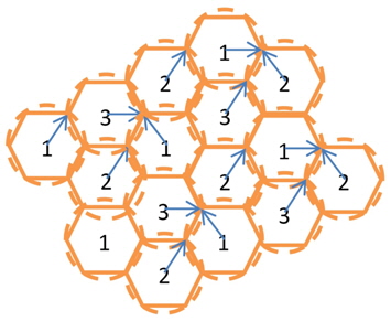
When planning a radio network, one implementation uses a homogenous structure of BSs [9-11]. An illustration of these structure is shown in Figure 1. In practice, factors such as the lie of the ground, subscribers’ density, automobile noise, the height of the buildings necessitate the use of a heterogeneous structure of BSs.
However, problem can arise when installing BSs with different structures. During the planning of heterogeneous BSs, additional interference or uncovered areas can occur, as shown in Figure 2. Our goal is to offer a solution to these problem(i.e., to minimize interference and prevent uncovered areas).
BS locations, another vital issue is frequency assignment. To avoid interference among new mobile technologies, neighboring cells should use different frequencies [12]. In Figure 1 and 2, the number in the center of the clusters indicates the frequency.
3.1 Heterogeneous Networks and Their Requirements
Heterogeneous networks are being used in a variety of areas: cellular telecommunications is a high-profile example, but they are also being used in many other areas, particularly where ad-hoc networks are being deployed. The network must be structured in such a way that the performance, as seen in all areas of the network, meets the requirements. Aspects such as latency, performance and speed must meet the requirements throughout the network[1].
With the challenges facing operators increasing user demanding for improved performance and lower costs, operators will be required to use an ever wider array of technologies to ensure satisfactory operation of their networks in a variety of scenarios.
To provide not only coverage, but the correct form of coverage in terms of small and macro cells, operators deploy a variety of types of base station; they must also implement a heterogeneous format for the backhaul.
With over 60% of traffic occurring within urban areas it is necessary to deploy a blend of macro cells and metro(i.e., small) cells in the environment. Because city planners want to keep the visual impact to a minimum, towers and masts are much less desirable for use in base stations. Unobtrusive small cells will be deployed alongside Wi-Fi to provide the required coverage. All of these systems must operate seamlessly as far as the user is concerned[2].
3.2 Radio Wave Propagation Models
Simulation of propagation is based on the prediction average received signal level at a given distance from the emitter; its dispersion values are based on the situation in the radio communication area. The radio coverage area of the transmitter can be determined by calculations. Simulation of the average signal based on the distance between the transmitter and the receiver is called large-scale simulation, because it allows one to determine the signal over long distances (several hundred or thousand feet). On the other hand, the other model is characterized by rapidly changing the values of the received signal level at small displacements (several wavelengths), or for a short time (several seconds); these are called small-scale models.
A model of wave propagation in free space is used to calculate the received signal in the case of the transmitting and receiving antennas located in a radio communication area free of obstacles. This model is used to analyze radio communication via satellite and terrestrial radio links operating at microwave frequencies (3 to 30 GHz).
When a radio wave propagates in free space, the output power of the receiving antenna, which is expressed as a function of the distance to the transmitting antenna, and the gain of the transmitting and receiving antenna.
When using this equation, it is assumed that the receiving antenna is located at a distance from the transmitter that corresponds to the far field (the Fraunhofer zone).
The space equation is often expressed in relation to a reference point located in the Fraunhofer zone. The reference distance is usually chosen to be 100 m or 1 km for communication over open countryside.
One of the most important characteristics of the communication channel is its signal propagation attenuation. The free space attenuation (in dB) in the Fraunhofer zone is determined by the expression
A different form of convenient attenuation in free space is in equation (2):

where

The path loss, representing the attenuation suffered by the signal as it travels through the wireless channel is given by the difference of the transmitted and received power in dB and is expressed as:

The fields of an antenna can broadly be classified in two regions, the far field and the near field. It is in the far field that the propagating waves act as plane waves and the power decays inversely with distance. The far field region is also termed as the Fraunhofer region and the Friis equation holds in this region. Hence, the Friis equation is used only beyond the far field distance,

Also we can see that the Friis equation is not defined for

Propagation models that estimate the average signal power for different distances between transmitter and receiver, from several hundred to several thousand meters, are called large-scale propagation models. Large-scale models are very simple and do not take into account very small changes, such as attenuation due to multipath propagation. These models are useful for predicting the coverage of radio systems[1,2].
3.2.1 The Okumura model
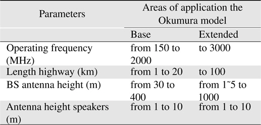
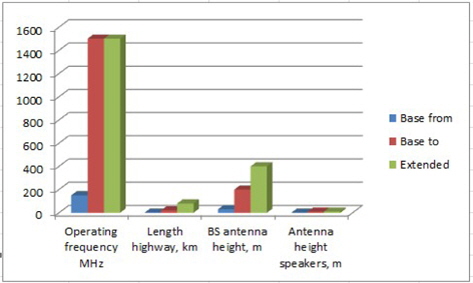
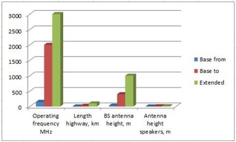
The Okumura model is based on a graphical representation of experimental data obtained for signal level measurement in Tokyo. This experimental approach is a widely used method for the calculation of radio information in a city. The Okumura model is used for the parameter values in the range indicated in Table 1 and Figure 3.
[Table 1.] Parameter values for the Okumura model

Parameter values for the Okumura model
The Okumura model based on the results of experimental studies (and compared with the two-beam model) can more accurately predict the average value of the attenuation of radio signals at a relatively long distance between the transmitting and receiving antennas (over 1 km) in the presence of obstacles.
According to the model, the average attenuation in dB is defined. Formula for Okumura model is expressed below:
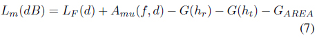
Where; Lm = (i.e., median) of path loss LF (d) = free space propagation path loss. Amu(f,d) = median attenuation relative to free space G(hb) = base station antenna height gain factor G(hm) = mobile antenna height gain factor G(hb) = 20log(hb/200) 1000 m > hb> 30 m G(hm) = 10log(hm/3) hm<= 3 m G(hm) = 20log(hm/3) 10 m > hm > 3 m
Figure 3 shows the result of Table 1. The left and middle ones of 3 bars are base parameters, the right one is extended parameter.
3.2.2 Hata model
The above model is inconvenient for calculations by a computer. Hata established empirical mathematical relationships to describe the graphical information given by Okumura. Hata’s formulation is limited to certain ranges of input parameters and is applicable only over quasi-smooth terrain. To increase the ease of implementation, Hata suggested an empirical model for describing graphical information provided by Okumura. Consequently, the Hata model (a mathematical notation) is also based on the experimental data from Okumura. The Hata model is used when changing parameter values within the limits specified in Table 2 and Figure 4.
[Table 2.] Possible values for the model parameters in the Hata model
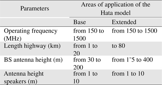
Possible values for the model parameters in the Hata model
Figure 4 shows the result of Table 2. The left and middle ones of 3 bars are base parameters, the right one is extended parameter.
Although, the Hata formula does not allow us to take into account all of the specific amendments that are available in the method of Okumura, it has significant practical importance.
3.2.3 Walfisch-Ikegami model
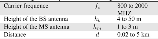
The Walfisch-Ikegami model is recognized as the best model for predicting signal information in small cells. This model is based on a physical representation of the field at the receiver in the form of two components: a coherent and a scattered component. The coherent component is determined using a wave diffract around the buildings along the road between BSs. The scattered component includes waves that are generated as a result of reconstruction of the incident wave from waves at the BSs. The scattered component includes directions that do not coincide with the direction of the BS and are even opposite to its direction. This model states, that, in a city with relatively low, densely spaced buildings, basic signal propagation (in the absence of direct line of sight [LOS] between nodes) is a path through the roofs of buildings (which can be described as a series of consecutive screens), followed by multiple scattering. The main parameters used in this model: transmission frequency (
Calculation formulas for Walfisch-Ikegami model are obtained for the following parameters: distance between the BS and BS of from 0.02 km to 5 km in the frequency range of 800 to 2000 MHz, a BS antenna height
[Table 3.] Range of validity for the Walfisch-Ikegami model

Range of validity for the Walfisch-Ikegami model
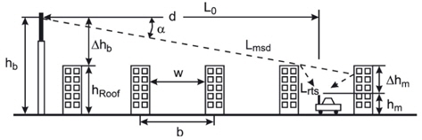
(1) In the LOS. To calculate the propagation loss using a relatively simple formula (2) Out of sight (none line of sight [NLOS]).
This case is more complicated. The amount by which the received signal strength decreases in passing from the source to the receiver is given by Figure 5.
The Walfisch-Ikegami model is a pathloss model for the case of small distances between MS and BS, and/or small height of the MS. The total pathloss for the LOS case is given by the equation (8).

For
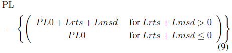
The free-space pathloss is the equation (10).

Ikegami derived the diffraction loss

is the difference between the building height
For the computation of the multiscreen loss

When designing small cells, we require information regarding specific areas of city roads. In some cases, one can use the statistics for the city: for a modern urban areas, building density is assumed to be 90 buildings per km2. The buildings’ average length is 80 to 105 m; their width is 15 m. Buildings have from 9 to 14 floors. The gaps between buildings 15 to 20 m. The average distance of LOS in a layer is 170 m. Garages can be considered homogeneous for areas in which there are no large open parks.
This study reviewed radio wave propagation models based on BS and antenna characteristics. Each model is described separately, in terms of their characteristics, parameters, and areas of application. The ideal distance at which to use the current model are determined. The model considers the current structure of the BSs. The research shows how these models affect the performance of mobile networks in different scenarios.