Figure/ground segmentation aims at partitioning an image into regions of coherent properties as a means for separating objects from their backgrounds. Considerable effort has been made to develop many advanced techniques in the recent years, where learning segmentation has attracted considerable attention of researchers because of its significant performance in classification applications. Further, probabilistic graphical models have also been remarkably successful in segmentation applications.
In any image system, feature representation is crucial to enhancing the system performance. How to manifest an image and how to capture salient properties of the object regions are still challenging problems. The bag-of-features (BoF) model [1-3] has been widely used in the field of image processing. The model treats an image as a collection of unordered appearance descriptors extracted from local patches, quantizes them into discrete ‘visual words,’ and then computes a compact histogram representation. In this work, we propose a patch-level BoF model to effectively represent an image patch from raw image data. By pixellevel dictionary learning, sparse coding, and spatial pyramid matching, the feature representation can capture the salient properties of the image patch, thus resulting in high patchwise segmentation accuracy.
Learning segmentation converts the image segmentation problem into a data clustering problem of image elements. One of the core challenges for machine learning is to discover what kind of information can be learned from the data sources and cluster this data into segments depicting the same object. Ren and Malik [4] proposed a classification model for segmentation, which feeds the Gestalt grouping cues into a linear classifier to discriminate between good and bad segmentation. Wu and Nevatia [5] developed a method to simultaneously detect and segment objects by boosting the edgelet feature classifiers. Duygulu et al. [6] modeled object recognition as a process of annotating image regions with words, and learning a mapping between region types and keywords by using an EM algorithm.
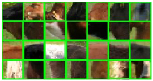
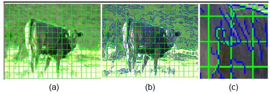
Probabilistic graphical models usually construct a cost function on the basis of some image constraints and formulate the image segmentation problem as a stochastic optimization problem. A condition random field (CRF) provides a principled approach to incorporating datadependent interactions; the complex joint probability distribution need not be modeled in this case. In this work, we use the CRF model to fuse multiple visual cues. For the CRF model, the definition of unary and pairwise potentials is very important. Previously, the unary potential was directly defined on feature spaces [7]. Lately, researchers have paid more attention on using a classifier to generate a unary potential [8-15], and most of them prefer using a pixel or a superpixel as the basic processing unit. In contrast, we use a regular image patch. Image patches on object boundaries contain rich local structure information of an object (see Fig. 1). While superpixels usually have a homogeneous appearance and an almost uniform size along with edge preservation, particularly for weak boundaries, these properties weaken the discriminative capability of the unary classifier when the superpixel is taken as the sampling unit.
Our main contributions in this paper are twofold. First, we use an image patch as a sample of a unary classifier and propose an upgrade patch feature representation based on pixel-level sparse coding, which can capture more structure information of the local contour of objects. Second, we propose the color and texture pairwise potentials with neighborhood interactions and an edge potential representing edge continuity, which are validated to be very effective in our experiments.
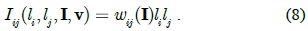
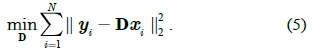
CRFs are probabilistic models for segmenting data with structured labels [16], which are defined on a twodimensional discrete lattice, every site on which corresponds to a graph node. Let
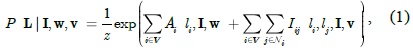
where
We use a CRF model to learn the conditional distribution over figure/ground labeling given an image, which allows us to incorporate different levels and different types of features in a single unified model.
In this work, the unary potentials are defined by the prediction probability obtained from a linear support vector machine (SVM) classifier. Different from the existing feature descriptions, we train a pixel-level over-complete dictionary to sparsely represent image patches in a highdimensional space.
1) Pixel-Level Texture Descriptor
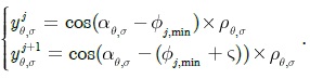
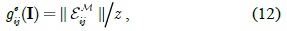
Gabor wavelets have received considerable attention because of biological reasons and their optimal resolution in both frequency and spatial domains. The Gabor wavelet representation can capture the local structure corresponding to the spatial scale, spatial localization, and orientation selectivity. It can characterize the spatial frequency structure in the image, while preserving the information of spatial relations. However, many existing image representation approaches in the Gabor domain merely consider the magnitude information. In this work, we proposed a new pixel-level feature descriptor, which fuses the Gabor magnitude and the Gabor phase.
To eliminate local noise interference, a simple smoothing filter is used for removing image noise in advance. Then, we perform the Gabor transform in

where
An example of diagram
We concatenate all vectors
2) Pixel-Level Dictionary Learning and Coding
Sparse representations have demonstrated considerable success in numerous applications, and the sparse modeling of signals has been proven to be very effective in signal reconstruction and classification. We randomly sample some pixels from the training image set to learn an over-complete pixel-level dictionary. Assuming that we collect N training samples, we define a matrix Y ∈ R
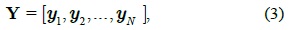
where
Using an over-complete dictionary D ∈ R
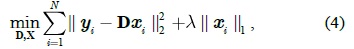
where
The optimization problem is convex in D or X while fixing the other, but not in both simultaneously [17]. We solve it by alternating the optimization over D and X ; the dictionary D can be initialized by randomly sampling

Once the over-complete dictionary D is given, the texture feature

3) Patch Feature Representation
The pivotal role of the unary potential in the CRF-based segmentation model has been demonstrated. It can be taken as a local decision term, which decides the association of a given graph node to a certain class. Usually, the use of the unary classifier alone leads to high accuracy as compared to the full CRF model as it can segment most parts of an object and loses only some details of the object boundaries.
In this work, we integrate the texture feature and the color feature to represent an image patch. We partition a patch into 1×2, 2×2 segments in two different scales, and then, compute the max pooling vector of the sparse codes of pixels within each of the five segments. We finally concatenate all the vectors to form a vector representation of the texture feature. The so-called spatial pyramid matching has had remarkable success in image classification applications. Color information is very useful for identifying the classes of image patches. For example, backgrounds (e.g., sky, water, grass, and tree) are usually distinguishable from objects (e.g., cow, sheep, and bird) in color. For a patch, we compute 64-bin histograms in each CIE Lab color channel as its color feature and then, concatenate the texture vector and the color vector to form the final feature representation. In our experiments, we fixed the size of dictionary D as 2048; thus, the dimension of the patch feature is 2048×5+64×3 =10432 . We also find that max pooling outperforms the other alternative pooling methods.
4) Unary Potential Computation
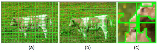
We train a binary linear SVM classifier to predict the figure/ground probabilities of an image patch, which are used for computing the unary potential. However, the boundaries of the foreground segmented by the CRF model using patches as graph nodes have a blocking effect. To generate results close to the ground truth, we split patches into some perceptually meaningful entities by using the over-segmentation boundary map, which is generated by an existing region merging method [18]. As shown in Fig. 3, a patch is split into several regions. These regions are considered the graph nodes, and their unary potential values are defined as the corresponding prediction probability of the host patch. That is, the regions split from a patch are assigned the same probability. In particular, the unary potential in Eq. (1) is defined as follows:

where
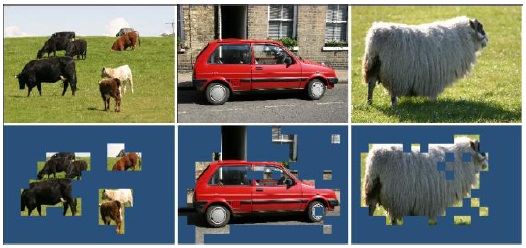
After the unary binary classification, we can already obtain good segmentation results, but the classifier separately processes each image patch. The mutual dependence among neighboring patches is ignored, which results in some neighboring patches with a similar appearance being possibly improperly labeled as opposite classes (see Fig. 4). Therefore, as contextual knowledge is necessary for image segmentation, we define the pairwise potential to address this problem. In this work, the pairwise penalty
In image segmentation, the weights encode a graph affinity such that a pair of nodes with a high weight edge is considered to be strongly connected and edges with low weights represent the nearly disconnected nodes. We exploit the color, texture, and edge cues to model the connection between nodes and incorporate the three types of potentials in a unified CRF framework using pre-learned parameters. Assuming that the superscripts

where
1) Color Potential and Texture Potential
Color information is an essential and typical representation for images and is a key element for distinguishing objects. Mean and histogram are two common color descriptors. Mean only describes the average color component rather than the color distribution in a region. We use the CIE Lab histogram as a color descriptor for computing the color potential. Similarly, each channel is uniformly quantified into 64 levels, and then, three channels are concatenated to form a 192-dimensional color vector. The experimental comparison demonstrates that the histogram descriptor is more effective than the mean descriptor, increasing the overall pixel-wise labeling accuracy by 3.8%.
Every region in natural images is not isolated and is strongly connected with its adjacent regions. When computing it is unreasonable to only use the node pair (
where
Similarly, we can compute the texture potential Further,

where
2) Edge Potential
Inside a very small region, edge information basically indicates local image shape priors; the regions belonging to the same object often have strong edge continuities, which are described as the edge potential in this paper. As shown in Fig. 5, we find that there are many edges (blue lines) going through neighboring nodes. If two neighboring nodes are crossed by an edge, they very possibly belong to a visual unit and have the same figure/ground label. Motivated by this observation, we define the edge potential to capture the cue of edge continuity.
Given an image, we compute its binary gradient magnitude

Then, the edge potential is computed as follows:
where and

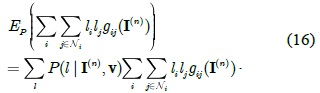
The parameter vector v in Eq. (7) is automatically learned from the training data. Given a set of training images T = {(L(
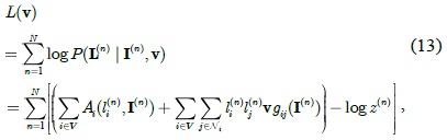
where the last term is the log-partition function. In general, the evaluation of the partition function is a NP-hard problem. We could use either sampling techniques (e.g., the Markov chain Monte Carlo method [19]) or some approximations (e.g., those of the free energy [20], piecewise training [21], pseudo-likelihood [22]) to estimate the parameters.
The optimal parameter maximizes the log conditional likelihood according to the CML estimation as follows:
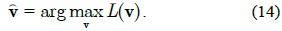
This can be solved by using the gradient descent method. The derivative of the log likelihood
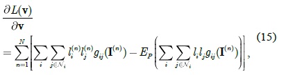
where the second term

In general, the expectation cannot be computed analytically because of the combinatorial number of elements in the configuration space of labels. In this work, we use belief propagation [23] to approximate it.
We evaluate the proposed approach using three datasets. The MSRC dataset [10] contains 591 images with 21 categories. The performance of the unary classifier on this dataset is measured by using the pixel precision. Furthermore, for comparison with a previous work [24], we select the following 13 classes of 231 images with a 7-class foreground (cow, sheep, airplane, car, bird, cat, and dog) and a 6-class background (grass, tree, sky, water, road, and building) as the data subset. The ground truth labeling of the dataset contains pixels labeled as ‘void’ (i.e., color-coded as black), which implies that these pixels do not belong to any of the 21 classes. In our experiments, void pixels are ignored for both the training and the testing of the unary classifier. The dataset is randomly split into roughly 40% training and 60% test sets, while ensuring approximately proportional contributions from each class.
The second dataset is the Weizmann horse dataset [25], which includes the side views of many horses that have different appearances and poses. We have also used the VOC2006 cow database [26] in which ground truth segmentations are manually created. For the two datasets, the numbers of images in the training and test sets are exactly the same as in [27].
When extracting the pixel-level texture descriptor, we set the parameters of the Gabor filter as scales
During the training of the unary classifier, a patch possibly contains multiple labels; however, we take the label that accounts for more than 75% of all the pixels in this patch as its label. We find that the number of patches of the training images in each class on average is in the order of 10000, and some classes have more than 100000 patches. Considering the memory and computational constraints, we randomly select 8000 patches from each class to construct a patch dataset for the evaluation of the unary classification, and each class sample is randomly split into 25% training and 75% test sets. For efficiency, we reduce the dimension of a patch feature from 10432 to 4000 by using the incremental principal component analysis (PCA) algorithm [28], in which we feed 20% samples to increment PCA in order to approximate the mean vector and the basis vectors.
To evaluate the performance of the proposed patch representation, we use a simple linear SVM classifier to conduct 21-class classification experiments on the MSRC dataset. We select 1200 patches per class as training samples and the rest of the patches as the testing samples. We achieve patch-wise labeling accuracy of 71.0%, while the state-of-the-art approach [10] gives pixel-wise accuracy of 69.6%. For a fair comparison, we further refine the patch precision segmentations to the pixel precision ones by simply post-processing.
In particular, we first get split patches (i.e., graph nodes) by using an existing segmentation method as described in Section III-A. The nodes are not always larger than the patches in size. Then, we take the nodes within the same segment as generated by [18] as the content consistent nodes. Finally, the label of each node is decided by a majority vote of the labels of its neighboring nodes, which must also be its content-consistent nodes. After the above processing, we achieve pixel-wise accuracy of 72.1%.
We also evaluate the binary classification performance on the 13-class dataset. We select 2200 patches per class as the training samples and label the 7-class foreground and the 6-class background as positive samples and negative samples, respectively. Thus, we achieve patch-wise labeling accuracy of 87.5%. After the post-processing, we achieve pixel-wise accuracy of 88.4%. The unary pixel-wise accuracy on the Weizmann dataset and the VOC2006 dataset is 89.9% and 94.5%, respectively.
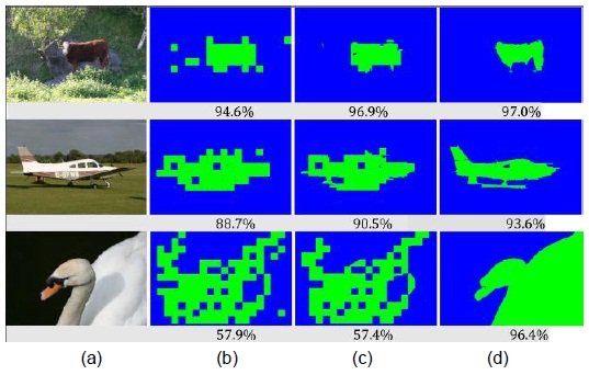
On the 13-class dataset, we compare the unary potential accuracy with the full model accuracy. The latter is improved by 3.2% on average. This seemingly small numerical improvement corresponds to a large perceptual improvement (see Fig. 6), which shows that our pairwise potentials are effective.
We evaluate the performance of the proposed method against that of three state-of-the-art methods [24,27,29]. The quantitative measure is the accuracy, namely segmentation cover, which is defined as the percentage of correctly classified pixels in the image (both foreground and background) [24,29].
On the MSRC dataset, since the performance varies substantially for different classes, we respectively give the accuracy of each class. We list the quantitative comparison of seven classes in Table 1, which shows that our method outperforms the two competitors except for the cat class.
[Table 1.] Quantitative comparison on the MSRC dataset
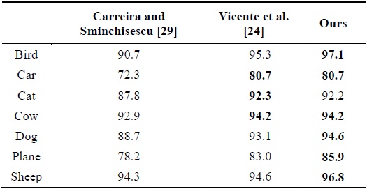
Quantitative comparison on the MSRC dataset
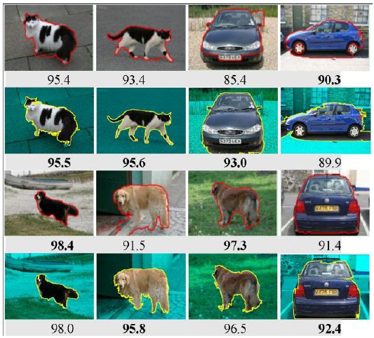
In addition, the method proposed in [24] only selects 10 images for each class such that there is a single object in each image, while we compute the segmentation accuracy on the 13-class sub-dataset of 231 images, and many images contain several object instances. The difference in testing data also indicates that our method is more robust than that proposed in [24]. Fig. 7 shows some visual examples of the same images as reported in [24]. Although the accuracies of some examples are lower than those in the case of the competitor methods, our overall accuracy is higher.
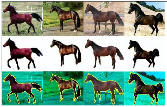
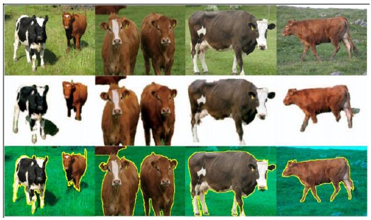
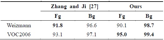
On the Weizmann and VOC2006 datasets, we compute the 2-class confusion matrix, as shown in Table 2, which shows that the proposed method performs favorably against the method proposed in [27] on the first dataset and much better on the second one. Figs. 8 and 9 show the same examples as those considered in [27]. The reason that the results on the cow dataset are very goodies that the appearances of the foreground and background are respectively homogeneous and the spatial distribution of the foreground is very compact. Compared to the horse dataset, the foreground of many images are inhomogeneous; in particular, horse shanks are very slim and their colors are different from those of the body, which leads to horse shanks going missing from the final segmentation, as shown in Fig. 8. In addition, the similar appearance of the foreground and the shadow in the background possibly causes some errors.
[Table 2.] Quantitative comparison on the Weizmann and VOC2006 datasets

Quantitative comparison on the Weizmann and VOC2006 datasets
In this paper, we propose a new discriminative model for figure/ground segmentation. First, a pixel-level dictionary is learnt from mass pixel-wise Gabor descriptors; second, each pixel is mapped as a high-dimensional sparse vector, and then, all the sparse vectors in a patch are fused to represent the patch by max pooling and spatial matching. The proposed unary features can simultaneously capture the appearance and context information, which significantly enhances the unary classification accuracy. The upgrade color and texture potentials with neighborhood interactions and the proposed edge potential weaken the interference of abnormal nodes during graph affinity computation. The experimental results demonstrate that the proposed approach is powerful with a comparison with three state-of-the-art approaches. In the future, we hope to integrate explicit semantic context and salient information to make the algorithm more intelligent.


![Qualitative comparison with [24] for the MSRC database. The first and the third rows show the results reported in [24]. The second and the fourth rows show our results.](http://oak.go.kr/repository/journal/17085/E1ICAW_2015_v13n3_205_f007.jpg)
![Examples of representative segmentation results on the Weizmann horse dataset. From top to down: input images, results reported in [27], and our results.](http://oak.go.kr/repository/journal/17085/E1ICAW_2015_v13n3_205_f008.jpg)
![Examples of representative segmentation results on the VOC2006 cow images. From top to down: Input images, results reported in [27], and our results.](http://oak.go.kr/repository/journal/17085/E1ICAW_2015_v13n3_205_f009.jpg)