Ion trap mass spectrometry has been developed through several stages to its present situation of relatively high performance and increasing popularity. Quadrupole ion trap (QIT), invented by Paul and Steinwedel,1 has been widely applied to mass spectrometry,2-11 ion cooling and spectroscopy,12 frequency standards, quantum computing,13 and so on. However, various geometries has been proposed and used for QIT.14
An ion trap mass spectrometer may incorporate a Penning trap,15 Paul trap16 or the Kingdon trap.17 The Orbitrap, introduced in 2005, is based on the Kingdon trap.18 Also, the cylindrical ion trap CIT has received much attention in a number of research groups because of several merits. The CIT is easier to fabricate than the Paul ion trap which has hyperbolic surfaces. In addition, the relatively simple and small sized CIT make it an ideal candidate for miniaturization. Experiments using a single miniature CIT showed acceptable resolution and sensitivity, and limited by the ion trapping capacity of the miniature device.19-21
With these interests, many groups such as Purdue University and Oak Ridge National Laboratory have researched on the applications of the CIT to miniaturize mass spectrometer.22,23
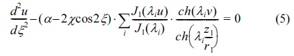
In CIT, the hyperbolic ring electrode,24 as in Paul ion trap, is replaced by a simple cylinder and the two hyperbolic end-cap electrodes are replaced by two planar end-plate electrodes.25 The potential difference applied to the electrodes24-26 is:
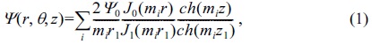
with

Where, U

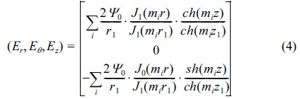
here, ▽ is gradient. From Eq.(3) (grad), the following is retrieved:
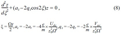
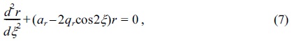
he equation of the motions10,21,24,25 of the ion of mass

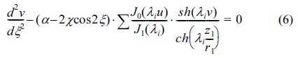
and the following

Where
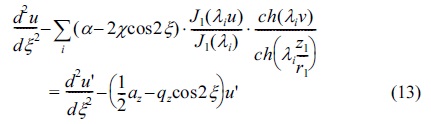
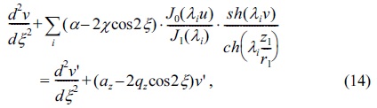
The motions of ion inside quadrupole ion trap
A hyperbolic geometry for the Paul ion trap was assumed;
Here,

CIT and QIT stability parameters
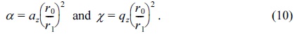
If the ions the same species are taken into consideration and the same potential amplitude and frequency, the following relations has been obtained:
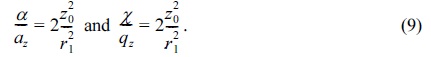
From Eq.(9) and one can obtain

The optimum radius between cylindrical ion trap and quadrupole ion Trap
In some papers,21,24 stability parameters have been used to determine the optimum radius size for cylindrical ion trap compared to the radius size for the quadrupole ion trap, as following:


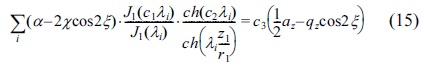
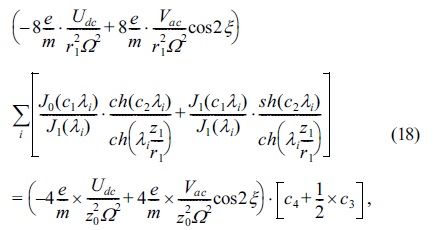
Eqs.(11) and (12) are from Refs,21,24 respectively. In this study, Eqs.(5), (6) and Eqs.(7), (8) were used for the same propose to find optimum radius size for cylindrical ion trap compared to the radius size for quadrupole ion trap, as:
with

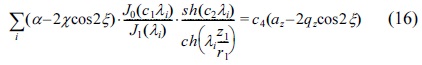
In adding Eqs.(15)and (16), we have:
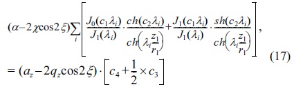
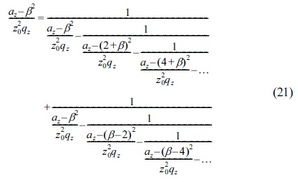
After substituting

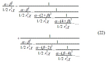
with Eq.(18) gives the optimum value of
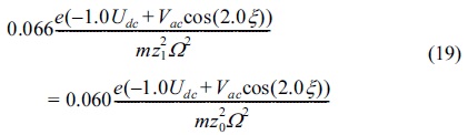
Therefore, using the Maple software we will have,

In Eq.(20),
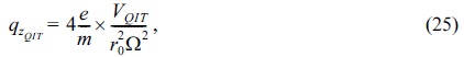
There are two stability parameters which control the ion motion for each dimension
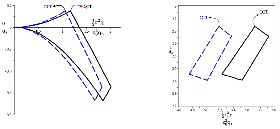
Figure 1 (a) and (b) shows the calculated first and second stability regions for the quadrupole ion trap and cylindrical ion trap,31) black line (solid line): QIT and blue line (dash line): CIT with optimum radius size
Figure 2 shows evolution of different values of the phase ion trajectory for
The results illustrated in Figure 2 show that for the same equivalent operating point in two stability diagrams (having the same
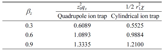
The values of for the quadrupole ion trap and cylindrical ion trap when az = 0 and α = 0 with z0 = 0.82 cm and optimum radius size z1 = 1.04985z0 and for βz = 0.3,0.6,0.9

and
for QIT and CIT, respectively. Hence, it is important to know that
>
The effect of optimum radius size on the mass resolution
he resolution of a quadrupole ion trap9 and cylindrical ion trap mass spectrometry in general with optimum radius size
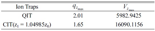
Table 2 shows the values of

The values of qzmax and Vzmax for the quadrupole ion trap with optimum radius size z1 = 1.04985z0, respectively in the first stability region when az = 0
when
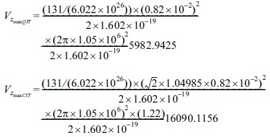
To obtain the values of Table 2 we suppose
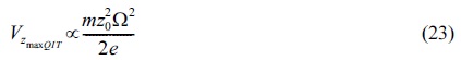
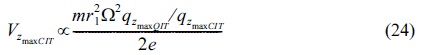
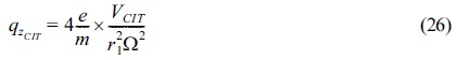
Now, we use Eqs.(23) and (24) to calculate

To derive a useful theoretical formula for the fractional resolution, one has to recall the stability parameters of the impulse excitation for the QIT and CIT with
By taking the partial derivatives with respect to the variables of the stability parameters
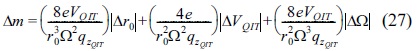
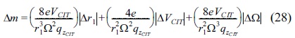
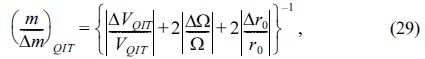
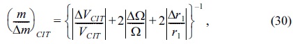
Now to find the fractional resolution we have,


Here Eqs.(29) and (30) are the fractional resolutions for QIT and CIT with optimum radius size
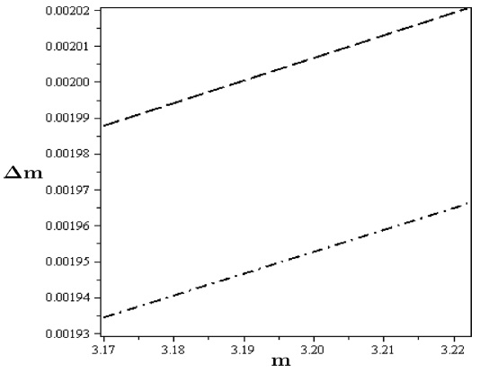
For the fractional mass resolution we have used the following uncertainties for the voltage, rf frequency and the geometry; ∆
In this study, the behavior of the quadrupole and cylindrical ion traps with the optimum radius has been considered. Also, it is shown that for the same equivalent operating point in two stability diagrams (i.e. having the same
Table 1 also indicate that for the same equivalent operating point, almost a comparison physical size between two ion traps are shown;
This difference in trapping parameters indicates that for the same rf and ion mass values, we need more confining voltage for CIT than QIT (see Table 2). So, higher fractional resolution can be obtained; higher separation confining voltages, especially for light isotopes9,31 (see Figure 3).