Sequences or time-series data are parts of our everyday life in diverse forms such as videos of image frames, speech signals, financial asset prices and meteorological records, to name a few. Sequence classification involves automatically assigning class labels to these instances in a meaningful way. Owing to the increasing demand for efficient indexing, search, and organization of a huge amount of sequence data, it has recently received significant attention in machine learning, data mining, and related fields. Unlike conventional classification of non-sequential vectorial data, sequence classification entails inherent difficulty originating from potentially variable-length and non-stationary structures.
Recent sequence classification approaches broadly adopt one of the two different frameworks. In the first framework, one estimates the similarity (or distance) measure between pairs of sequences, from which any kernel machines (e.g., support vector machines) or exemplarbased classifiers (e.g., nearest neighbor) can be employed. As the sequence lengths and sampling rates can differ from instance to instance, one often resorts to warping or alignment of sequences (e.g., dynamic time warping), alternatively, incorporating a specially-tailored similarity measure (e.g., spectral or string kernels [1]).
The second framework is based on probabilistic sequence models, essentially aiming to represent an underlying generative model for sequence data. The hidden Markov model (HMM) is considered to be one of the most popular sequence models, and has previously shown broad success in various application areas including automatic speech recognition [2, 3], computer vision [4–6], and bioinformatics [7]. y-based one in several aspects: certain statistical constraints such as Markov dependency structures can be easily imposed. In addition, the model-based approaches are typically computationally less demanding for training, specifically linear time in the number of training samples, while similarity-based methods require quadratic. Thus, throughout the study we focus on HMM-based sequence classification: the details of the model are thoroughly described in Section 2.
Unlike the traditional learning setup where all the labeled training samples are stored and available to a learning algorithm (i.e.,
Considering the cost of obtaining class labels, which typically requires human experts endeavor, the online learning algorithms can be more favorable. Moreover, they are better suited for various applications, most notably the mobile computing environments, in which there are massive amount of data collected and observed whereas the computing platforms (e.g., mobile devices) have minimal storage and limited computing power. It is worth noting that the online selective-sample learning setup is different from the well-known active learning [8, 9] in machine learning. In the active learning, the algorithm has full access to entire data samples (thus requiring data storage capabilities), and the goal is to output a subset for which the class labels are queried. In this sense, the online selective-sample learning can be more realistic and challenging than the active learning.
Recently there have been attempts to tackle the online selective-sample learning problem. In particular, the main idea of the latest aggressive algorithms (e.g., [10, 11]) is to decide to query labels for samples that appear to be novel (compared to the previous samples) with respect to the current model. Moreover, it is desirable to ask for labels for those data that have less confident class prediction under the current model, which is also intuitively appealing. However, most approaches are limited to vectorial (non-sequential) data and binary classification setups with the underlying classification model confined to the simple linear model.
We extend the idea to the multi-class sequence data classification problem within the HMM classification model. Specifically, we deal with the negative data log-likelihood of the incoming sequence as a measure of data novelty. Furthermore, the entropy of the class conditional distribution given the incoming sequence is considered as a measure of strength/confidence in class prediction. The proposed approach is not only intuitively appealing, but also shown to yield superior performance to the baseline approaches that make queries randomly or greedily. These results have been verified for several sequence classification datasets/problems.
The paper is organized as follows: after introducing a few notations and a formal problem setup, we describe the HMM-based sequence classification model that we deal with throughout the study in Section 2. Our main approach is described in Section 3, and the empirical evaluations are demonstrated in Section 4.
1.1 Notations and Problem Setup
We consider a
In the online selective-sample learning setup, the learner receives a sequence one at a time, and decides whether to query its class label or not. More formally, at the
2. HMM-based Sequence Classification Model
We consider a probabilistic sequence classification model
The HMM is composed of two generative components: (i) a (hidden) state sequence s =
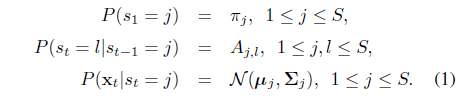
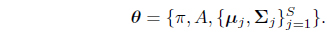
The parameters of the HMM are denoted by

In typical cases, the state sequence s is not observed, and one has to deal with the observation likelihood which is marginalization of the full joint likelihood over all possible hidden sequences, namely
While the parameter learning of the HMM can typically done by the EM algorithm
Returning to the classification model, we deal with
3. Online Selective-Sample Learning for SC-HMM
Our online selective-sample learning algorithm for the SC-HMM model is motivated from the aggressive algorithm of [11], and we briefly review their approach here. However, it should be noted that their approach is based on the simple linear model for binary classification of vectorial (non-sequential) data, hence should be differentiated from our extension.
In [11] a linear classification model
The model w is basically estimated by L2-regularized linear regression, which gives rise to the estimate w = A−1b at stage

Note that (3) can be computed/updated in an online fashion. Then the model’s score is computed as: . Whether to query
In their algorithm, due to the simple linear regression model and Gaussianity assumption, the query decision rule is easily derived and the update equation becomes simple. For sequence classification, the underlying model is a rather complex SC-HMM, and extension of the idea requires further endeavor. At each stage
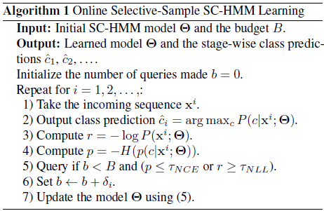
First, decision to query is made if the incoming sample meets either of two conditions with respect to the current model Θ. (Cond-1) − log
The second step is to update the model Θ using the current data sample. The true class label
In the batch learning case with
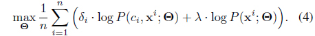
Here note that we can exploit even the unlabeled samples (the second term) by maximizing the marginal log-likelihood where the two objectives are balanced by the hyperparameter
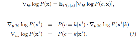
In the stochastic gradient ascent

which can be seen as an unbiased sample for the total gradient. The constant
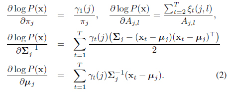
The nice thing is that (5), although derived from a batch setup, can be computed in an online fashion, and it exactly forms our model update equations. To be more specific to the SC-HMM, the gradients can be computed by (for each
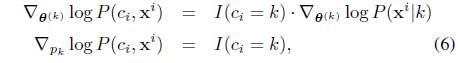
where

The initial model is chosen randomly and blindly, thus tends to select first a few samples for query, which is a desirable strategy considering that model is inaccurate with little labeled data received at initial stages. We stop the algorithm when the number of queries made reaches the budget constraint

In this section we evaluate the classification performance of the proposed online selective-sample learning algorithm on several real-world time-series datasets including human gait/activity recognition and facial emotion prediction. For each dataset we form online learning setups by feeding a learning algorithm one sample at each stage randomly drawn from the data pool, where we restrict the algorithm to make queries up to
Our algorithm is compared with two fairly basic online learning strategies: the first is to make queries at the first
As a performance measure, we accumulates the test errors up to
The classification task we deal with is to identify a person based on his/her gait sequence. We collect data from the speed-control human gait database
For
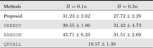
[Table 1.] Accumulated test prediction errors (%) on human gait recognition data

Accumulated test prediction errors (%) on human gait recognition data
It is also interesting to see that when the budget
4.2 Facial Emotion Classification
Next we consider the problem of recognizing facial emotion from a video sequence comprised of facial image frames that undergo changes in facial expression. From the Cohn-Kanade facial expression video dataset
For the sequence representation, we use certain image features extracted from images as follows. We first estimate the tight bounding boxes for faces using the standard face detector (e.g., Viola and Jones
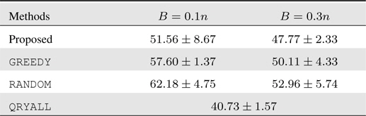
The test errors are depicted in Table 2, where the reference QRYALL again gives lower bound on the test errors. Our proposed method outperforms the competing methods significantly and consistently for all budget setups, while for
[Table 2.] Accumulated test prediction errors (%) on facial emotion classification data
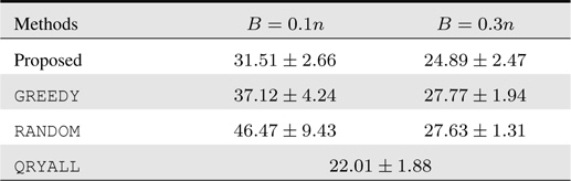
Accumulated test prediction errors (%) on facial emotion classification data
4.3 Human Activity Recognition
Last but not least, we tackle the problem of human activity recognition from a sequence of motion localization records. We obtain the dataset from the UCI machine learning repository
For this 3-way classification problem, we form online learning setups similarly as previous experiments. The test results are summarized in Table 3. We again have similar behavior as the former two experiments. The performance of the proposed approach is outstanding: in particular, it even attains more accurate prediction with the smaller budget constraint. In this dataset, due to the rather limited feature information, the overall prediction performance is low, and under such scenarios, the sophisticated query decision in our algorithm is shown to yield viable solutions.
[Table 3.] Accumulated test prediction errors (%) on human activity recognition data

Accumulated test prediction errors (%) on human activity recognition data
In this paper we have proposed a novel online selective-sample learning algorithm for multi-class sequence classification problems. Under the HMM-based sequence classification model, we devise reasonable criteria for decision for query based on the data novelty (likelihood of the incoming data) and the class prediction confidence (entropy of the class posterior). For several sequence classification datasets/tasks in online learning setups, we have shown that the proposed algorithm yields superior prediction accuracy to greedy or random approaches even with a limited query budget. One current issue may be how to choose the threshold parameters adequately, and we leave it as our future work to investigate a systematic way to tune those.