Artificial neural networks (ANNs) are nonlinear mapping structures based on the function of the human brain. They are powerful tools for modeling, particularly because the underlying data relationship is unknown. The key element of this paradigm is the novel structure of the information processing system. It is composed of a large number of highly interconnected processing elements (neurons) working in unison to solve specific problems. An ANN is configured for a specific application, through a learning process. Learning in a biological system involves adjustment to the synaptic connections that exist between the neurons. ANNs can identify and learn the correlated patterns between input datasets and the corresponding target values. After training, ANNs can be used to predict the input data. ANNs imitate the learning process of the human brain and can process problems involving nonlinear and complex data even if the data are imprecise and noisy. Thus, they are ideal for the modeling of complex and often nonlinear data. ANNs have great capacity for predictive modeling; i.e., all the characters describing the unknown situation can be presented to the trained ANNs, and then, the prediction of systems is guaranteed. ANNs are capable of performing many classification, learning, and function approximation tasks, yet in practice, they sometimes deliver only marginal performance. Inappropriate topology selection and weight training are frequently blamed for this. Neural networks are adjusted, or trained, such that a particular input leads to a specific target output. The ANN weights are adjusted on the basis of a comparison of the output and the target, until the network output matches the target. Typically, many such input/target pairs are needed to train a network. Increasing the number of hidden layer neurons helps to improve the network performance, yet many problems can be solved with very few neurons if only the network takes its optimal configuration. Unfortunately, the inherent nonlinearity of an ANN [1] results in the existence of many suboptimal networks, and a considerable majority of training algorithms converge to these suboptimal configurations. The problem of multiple local minima in neural networks has been widely addressed. The proposed solutions include multiple starts from randomly chosen initial points, simulated annealing, random perturbation, diffusion techniques, and evolutionary computing. Most of these methods are probabilistic in nature: They can find the globally optimal solution with a certain probability, which depends on the number of iterations of the algorithm. In this study, an ANN is trained using the proposed hybrid approach. The rest of this paper is organized as follows: Section II presents a brief introduction to different existing ANN learning algorithms with their pros and cons. The proposed hybrid DPSO-BP approach is introduced in Section III. Simulation results and comparisons are provided in Section IV to demonstrate the effectiveness and potential of the proposed hybrid algorithm. Finally, several conclusions are presented in Section V.

Training neural networks is a complex task of great importance in the field of supervised learning. ANNs have been shown to have the potential to perform well for classification problems in many different environments, including business, science, and engineering. A majority of the studies on this topic rely on a gradient algorithm, typically a variation of backpropagation (BP), to obtain the weights of the model. Various learning techniques are introduced to optimize the weights of an ANN. Although the limitations of gradient search techniques applied to complex nonlinear optimization problems, such as the ANN, are well known, many researchers still choose to use these methods for network optimization. ANNs can identify and learn the correlated patterns between input datasets and the corresponding target values. After training, ANNs can be used to predict input data. ANNs imitate the learning process of the human brain and can process problems involving nonlinear and complex data even if the data are imprecise and noisy. Different learning algorithms are described below.

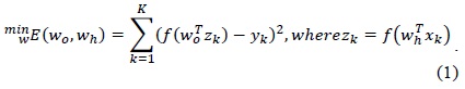
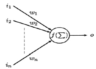
In an ANN, activation functions of the output units become differentiable functions of the input variables and of the weights and biases, as shown in Fig. 1. If we define an error function (E), such as a sum of squares function, which is a differentiable function of the network outputs, then this error function is itself a differentiable function of the weights. We can therefore evaluate the derivatives of the error with respect to the weights, and these derivatives can then be used to find the weight values that minimize the error function, by using any of the learning algorithms such as the BP, conjugate gradient, quasi-Newton, and LevenbergMarquardt (LM) algorithms [2]. From the perspective of mathematical programming, supervised batch training of a neural network is a classical nonlinear optimization problem: find the minimum of the error function given some set of training data. Traditionally, this is accomplished by a suitable local descent technique, such as BP. The independent variables are the weights w, and the objective function is usually the sum of squared errors (although other measures of error are also used). The objective function is formulated mathematically in Eq. (1).

Here, f denotes the transfer function; w_o, the output weights; w_h, the hidden layer weights; x_k, the input training data; y_k, the desired output; and z_k, the activations of hidden neurons. Despite its popularity, BP has been widely criticized for its inefficiency, and more advanced minimization techniques, such as conjugate gradient and LM methods, are available. Yet, all these techniques converge to the closest local minimum of the error function, which is very unlikely to be the global one. As a consequence, a network trained with a local algorithm may exhibit marginal performance. In this connection, the primitive BP may result in a better solution than more sophisticated methods, because its disadvantages turn into the benefits of avoiding some shallow local minima. Thee problem of many local minima has been widely addressed in the past. It was shown that training even a simple perceptron with a nonlinear transfer function may result in multiple minima. The remedies include starting the local descent from several random points, using tabu search, simulated annealing, and genetic algorithms [3]. The new stochastic optimization algorithms significantly outperform the local methods, yet they do not provide any guarantee that their solution is the global minimum indeed. Moreover, thee number of local minima of the error function grows exponentially with the number of neurons, and the likelihood that these stochastic methods will find the global minimum is not very high.

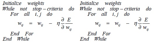
The BP algorithm is a classical domain-dependent technique for supervised training. It works by measuring the output error, calculating the gradient of this error, and adjusting the ANN weights [4] (and biases) in the descending gradient direction.

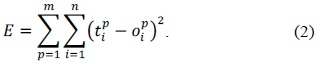
Hence, BPP is a gradient descent local search procedure (expected to stagnate in the local optima in complex landscapes). The squared error of the ANN [5] for a sset of patterns is calculated using Eq. (2).

The actual value of the previous expression depends on the weights of the network. The basic BP algorithm calculates the gradient of E (for all the patterns) and updates the weights by moving them along the direction of the gradient descent. This can be summarized with the expression △w = -η∇E, where the paramenter η > 0 is the learning rate that controls the learning speed. The pseudocode of the BP algorithm is shown in Fig. 2.

The particle swarm optimization (PSO) algorithm was first introduced by Kennedy and Eberhart [6]. Instead of using evolutionary operators to manipulate the individuals, as in the case of other evolutionary computational algorithms, each individual in the PSO flies in the search space with a velocity that is dynamically adjusted according to its own flying experience and its companions' flying experience. Each individua is treated as a volume-less particle (a point) in the D-dimensional search space. The i-th particle is represented as X_i = (x_il, x_i2, ..., x_iD). The best previous position (the position giving the best fitness value) of the i-th particle is recorded and represented as P_i = (p_il, p_i2, ..., p_iD). The index of the best particle among all the particles in the population is denoted by the symbol g_b representing the global best value. The index of the best position for each particle in the population is denoted by the symbol i_b representing the individual's best value. The rate of the position change (velocity) for particle i is represented as V_i in the following equation: (v_il, v_i2, ..., v_iD). The particles are manipulated according to the following equation.

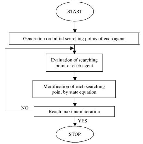
The algorithm can be summarized as follows (in Fig. 3):

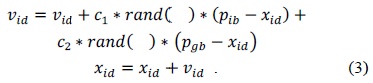
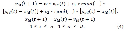
PSO-BP is an optimization algorithm combining PSO with BP [7,8].The PSO algorithm [9] is a global algorithm that has a strong ability to find the global optimistic result. However, this algorithm has a disadvantage that the search around the global optimum is very slow. In contrast, the BP algorithm has a strong ability to find the local optimistic result, but its ability to find the global optimistic result is weak. The fundamental idea for this hybrid algorithm is that at the beginning stage of searching for the optimum, PSO [10] is employed to accelerate the training speed. When the fitness function value has not changed for some generations, or the change in value is smaller than a predefined number, the search process is switched to the gradient descent search according to this heuristic knowledge. The PSO-BP [11] algorithm’s search process also starts by initializing a group of random particles. First, all the particles are updated according to Eq. (4).

where c₁ and c₂ are the acceleration constants with positive values and rand() is a random number between 0 and 1. Further, w is the inertia weight [12], until a new-generation set of particles is generated; then, these new particles are used to search the global best position in the solution space. Finally, the BP algorithm is used to search around the global optimum. Thus, this hybrid algorithm may find an optimum more quickly.

The procedure for this PSO-BP algorithm can be summarized as follows:

This algorithm has a parameter called the learning rate [13] that controls the convergence of the algorithm to an optimal local solution; however, obtaining a good value for this parameter is difficult.

PSO combined with BP gives good result in learning but due to some cons of basic PSO, we modified it with some dynamic constraints where during the learning process of the ANN objective space can be compressed or expanded. In PSO, each particle should be kept in a confined space corresponding to the parameter limitations. This decreases the diversity of the particle. If the global best particle does not change its g_best position after one iteration, then stagnation occurs in the population. Then, the solution may be a local optimal solution. That is, due to its stochastic behavior, it is not possible to find a way to the global optimum. The drawback of PSO is that the swarm may converge prematurely. The underlying principle behind this problem is that for the global best PSO, particles converge to a single point, which is on the boundary between the global best and the personal best positions. This point is not guaranteed for a local optimum. Another reason of this problem is the fast rate of information flow between particles, resulting in the creation of similar particles with a loss in diversity that increases the possibility of being trapped in the local optima. A further drawback is that stochastic approaches have a problem-dependent performance. This dependency usually results from the parameter settings in each algorithm. The different parameter settings for a stochastic search algorithm result in high performance variances. In general, no single parameter setting can be applied to all problems. Increasing the inertia weight (w) will increase the particle speed, resulting in more exploration (global search) and less exploration (global search). On the other hand, reducing the inertia weight will decrease the particle speed, resulting in more exploitation and less exploration. Thus, finding the best value for the parameter is not an easy task and may differ form one problem to another. Therefore, from the above, it can be concluded that the PSO performance is problem dependent. The problem-dependent performance can be addressed through a hybrid mechanism that combines different approaches in order to benefit from the advantages of each approach.

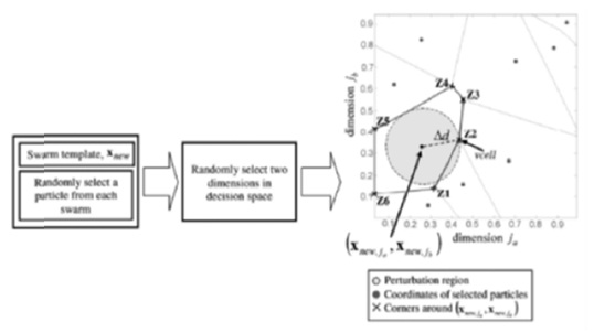
To overcome such limitations, a multiple-swarm PSO algorithm called dynamic multiple swarms in PSO is proposed in which the number of swarms is adaptively adjusted throughout the search process via d dynamic swarm strategy. The strategy allocates an appropriate number of swarms required to support the convergence and diversity criteria among the swarms. The main objective of this is to develop a multiple-swarm PSO that eliminates the need to estimate an initial number of swarms to improve the computational efficiency without compromising the performance of the algorithm. Once the swarm template (x_new) is generated, the template is perturbed to generate a swarm of particles. In order for perturbation to happen, the perturbation region centered around x_new needs to be defined; in addition to x_new, a particle from every swarm is randomly selected. For example, Fig. 4 shows eight randomly selected particles from eight different swarms in addition to x_new. The black circle in Fig.. 4 represents the coordinate of x_new, i.e., (x_new, j_a,x_new, j_b). Since there are more than two corners around the coordinate of x_new (i.e., represented by the 'x' symbol and labeled as Z1-Z6 in Fig. 4), a corner is randomly selected. In Fig. 4, the selected corner is Z2 and is denoted as v. The distanced between the center ans Z2, i.e., D, is computed to form the perturbation region of x_new. The proposed algorithm, DPSO, involves two key strategies: a swarm growing strategy to allocate more swarms if necessary and justified, and a swarm declining strategy to eliminate swarms that fail to contribute in the search of a Pareto front. Additional designs are included to support the aforementioned two strategies. These designs include the following:

In DPSO adding and removing the swarms throughout the search process will directly affect the swarm population distribution. Instead of applying the Pareto ranking method to update the Pareto rank of the particles and applying a niching strategy to estimate the density of the particles when the swarm population progresses at every iteration.

In the DPSO-BP algorithm, to know when the search process is transited from the particle swarm search to the gradient descent search, a heuristic way was introduced.

That is, when the best fitness value in the history of all particles does not change for some generations (i.e., ten generations), the search process is transferred to the gradient descent search. When the best fitness does not change for some generations, all the particles may lose the ability to find a better solution; at this time, a gradient descent search can be used to obtain better results. If the rank values of a current swarm and its recorded swarm leader have the same rank value, then the pure Pareto ranking method is applied to both the swarm leaders. If the current swarm dominates the recorded swarm leader, then the current one will replace the recorded one. If both do not dominate each other, one of them is randomly chosen to update the local best archive of swarms. The new velocity and position are given in Eq. (5).

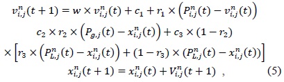
where is the j-dimensional velocity of swarm member i of swarm n in iteration t; the j-dimensional position of swarm member i of swarm n in iteration t; the j-dimensional personal best (p_best) position of the swarm members i of swarm n in iteration t; the j-dimensional global best (g_best) selected from the archive in iteration t; the j-dimensional local best position of the swarm leader of swarm n in iteration t; and (with a superscript the j-dimensional local best position of any swarm leaders other than their own swarm leader in iteration t. Further, r₁, r₂, and r₃ are random numbers within [0,1] that are regenerated every time they occur; w is the inertial weight that varies between 0.1 and 0.5 at every iteration; and c₁, c₂, and c₃ are the acceleration constants. Each of the acceleration constants is randomly varied between 1.5 and 2 to place different emphasis on the components. When the objective space compression strategy [14] is applied several times in the early iterations, there is a possibility that the objective space is overly compressed and can cause the boundaries of the objective to not cover the true Pareto front.

We choose two different datasets of small and large dimensions for the experiment. It is assumed that the proposed hybrid learning algorithm works in both these environments. The datasets are the e-learning dataset (number of patterns = 90) and the thyroid dataset (number of patterns = 7,200).

In the following experiments, two datasets are chosen for comparing the performances of the BP, PSO, PSO-BP, and DPSO-BP algorithms in evolving the weights of the ANN. Suppose that every weight in the network was initially set in the range of [-50,50], and all thresholds in the network were 0 s. Further, suppose that every initial particle was a set of weights generated at random in the range of [0,1]. Let the initial inertial weight w be 1.8, the acceleration constants, both c₁ and c₂ be 2.0, r₁ and r₂ be two random numbers in the range of [0,1]. The maximum velocity was assumed as 10 and the minimum velocity as -10. The initial velocities of the initial particles were generated randomly in the range of [0,1]. After each iteration, if the calculated velocity was larger or smaller than the maximum velocity or the minimum velocity, velocity would be reset to 10 or -10. The population size was a variable that was set according to the dataset. In this example, we trained an ANN with the structure of 1–S1–1. The training algorithms used were the DPSO-BP, DPSO, and BP algorithms. Assuming that S1 = 3, 4, 5, 6, 7, x was obtained from the range of [0, p] and the training set was obtained at an identical sampling interval of 0.03 from [0, p]; further, the test set was obtained at an identical sampling interval of 0.1 from 0.02 to p. For every fixed hidden unit number, we ran the training algorithms for each dataset. We set the maximum number of training iterations at 7,000 times for the algorithms.

Algorithms for training ANNs were compared. Tests were conducted on gradient descent algorithms such as BP, and population-based heuristics such as PSO. Experimental results showed that DPSO–BP outperformed all other algorithms in training neural networks. In this study, the DPSO–BP algorithm, which is a new, simple, and robust optimization algorithm, was used to train the standard and e-learning datasets for classification purposes. Training procedures involved the selection of the optimal values of the parameters, such as the weights between the hidden layer and the output layer, spread parameters of the hidden layer base function, center vectors of the hidden layer, and bias parameters of the neurons of the output layer.

PSO and PSO-BP algorithms showed better performance than derivative-based methods; however, these algorithms had the disadvantage of a slow convergence rate. Trapping a local minimum was a disadvantage for these algorithms. When the learning performances were compared, experimental results showed that the performance of the proposed algorithm was better than that of the others.

The success of the classification results of the test problems was superior and correlated with the results of many research [9,10,12]. In real-time applications, the number of neurons might affect the time complexity of the system. The results of the e-learning classification problem were reasonable and might help training algorithms in other e-learning applications.

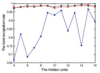
Fig. 5 shows the recognition rate of different algorithms while training an ANN in the thyroid dataset. Here, the red line denotes the proposed algorithm, while the blue and black lines denote the results of PSO and PSO-BP, respectively. It can be inferred from Fig. 5 that PSO-BP has a better recognition rate than PSO. Apparently, the PSO algorithm has a very low recognition rate while learning the ANN, but when it is combined with the BP algorithm, the mean recognition rate increases, as shown in Fig. 5. However, the proposed algorithm again increases the rate of recognition due to its dynamic nature. This shows that the DPSO-BP algorithm is more stable, while in the training process, the DPSO-BP algorithm uses less CPU time than the PSO-BP algorithm and the PSO algorithm.

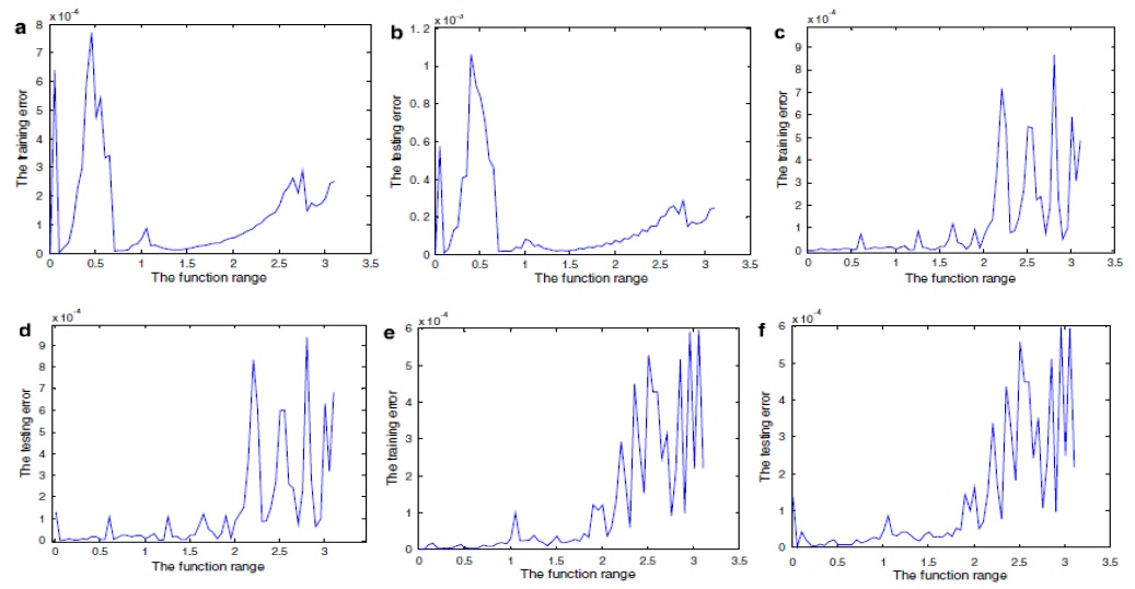
Fig. 6 illustrates the curves of the training errors and the testing errors for the three training algorithms using the elearning dataset. Fig. 6(a), (c), and (e) show the training error curves of the PSO, PSO-BP, and DPSO-BPA algorithms, respectively. Fig. 6(b), (d), and (f) illustrate the testing error curves of the PSO, PSO-BP, and DPSO-BPA algorithms, respectively. When the value of x is smaller, there are fewer training samples and testing samples. Further, it can be seen from Fig. 6 that the DPSO algorithm has better training and testing errors than the BP algorithm. When the value of x is larger, there are more training samples and testing samples. Moreover, it can be seen that the BP algorithm has better training and testing errors. The hybrid algorithm combines the advantages of the DPSO algorithm and the BP algorithm; therefore, it can be observed that the DPSO-BP algorithm has better training and testing errors.

In this paper, a hybrid DPSO-BP algorithm is proposed, which combines the PSO algorithm’s strong ability of global learning and the BP algorithm’s strong ability of local learning. Hence, we can obtain better training results by using this hybrid algorithm. Some heuristic knowledge is adapted to transit from the DPSO algorithm search to the BP algorithm search. That is, when the best fitness value in the history of all particles does not change for some generations (i.e., ten generations), the search process is transferred to the gradient descent search. The heuristic way is used to avoid wasting too much CPU time on a vain search (as used in the other compared algorithms); therefore, the training efficiency of the DPSO-BP algorithm is improved considerably. A different selection strategy is introduced for updating the inertial weight w. In the initial searching stage, the searching inertial weight is reduced rapidly in order to rapidly achieve the global optima. Then, around the global optimum, we reduce the inertial weight more smoothly by using BP so that a higher accuracy can be achieved.

From the conducted experiments, we conclude that for the same goal, the DPSO-BP algorithm uses less CPU time and provides higher training accuracy than the PSO algorithm and the BP algorithm. A comparative study shows that the performance of the variant is competitive in comparison with the selected algorithms on standard benchmark problems. It is concluded that the DPSO-BP algorithm is more stable than the BP algorithm and the PSO algorithm. In future research works, we shall focus on how to apply this hybrid PSO algorithm to solve more practical problems.