Research related to renewable energy has been conducted in recent years owing to elevated interest in energy such as wind power, solar power, tidal current, and wave power because of the possible exhaustion of fossil fuels. Typically, wind power generation uses the following process: a turbine converts wind energy to mechanical energy, and generators convert mechanical energy to electric energy. The electricity produced by the generators is connected to the grid side by a power converter device [1].
A power converter device is composed of a back-to-back PWM converter that consists of two converters: a generator-side converter, which turns over the energy produced from generators to the grid; and a grid-side converter that consistently controls both the DC-link voltage and the power factor (PF). In the conventional method, the ripple that occurs from switching is eliminated by applying an L filter to the grid-side converter. However, the methods using an L filter have disadvantages. For example, when a small L filter is used, it generates EMI in the device connected to the grid. If a large L filter is used, it increases the device volume and price, and worsens the dynamic characteristics. Therefore, an LC filter and an LCL filter are introduced by combining L and C. The LCL filter can produce excellent filter effects by using a small L filter. However, it makes the PF of the grid side worse owing to a resonance problem and a reactive current from the grid side to the filter capacitor [1-3].
There are various ways to solve these resonance problems. Generally, the resonance is removed by combining a damping resistor with the filter capacitor serially [4, 5]. However, the damping resistor causes loss, lowering the efficiency of the system. Thus, various active damping methods have been proposed. Considering that active damping methods control the current so that it has the difference of 180° status of the resonance components, it is required to satisfy the excellent dynamic characteristics of control. If the low dynamic characteristics cannot make the phase fit, serious problems can cause the system to diverge.
In order to control the PF of the grid side, it is necessary to have a controller that provides reactive current from the converter side provided from grid side to the filter capacitor. It is possible to calculate the value of the reactive current provided to the filter capacitor. However, if it is possible to determine the grid current, then effective control of the PF of the grid side is possible by controlling the reactive current of the grid current at zero and letting the converter provide reactive current to the filter capacitor.
The grid current ought to be informed in order to control the PF of the active damping and the grid side. In order to determine the current of the grid, it is possible to estimate the grid current by adding a current sensor or designing an observer. The two representative methods for estimating the grid current are as follows: first, use the converter current and the filter capacitor voltage; second, design the observer by applying a Kalman filter [6, 7]. However, since the method that uses a Kalman filter needs a significant operational quantity, a method for reducing the operational quantity is required.
This paper combines feedback linearity with a sliding mode control to remove the nonlinearity of the system and increase the response of the control. In addition, in order to decrease the operation quantity, the sensor is not added with estimating the grid current and applying a suboptimum observer.
Section 2 explains the modeling of the LCL filter. Section 3 describes the FL-SMC resonant control with an observer as follows: Section 3.1 explains feedback linearization, Section 3.2 explains the sliding mode control, Section 3.3 explains the determination of the stability in the controller, and Section 3.4 explains the suboptimum observer. Section 4 shows the results of the simulation. Finally, Section 5 presents the conclusion.
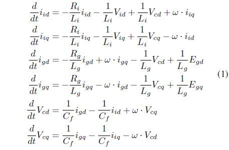
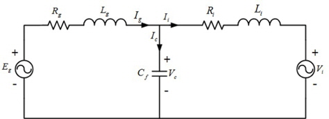
Figure 1 is an equivalent circuit of the LCL filter, and it can be expressed in voltage equations as follows [8]:

where
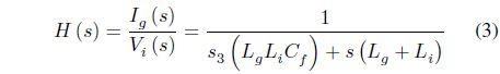
The transfer function between the converter voltage and the filter capacitor can be expressed as follows [9], [10]:

The resistance component is ignored here, and
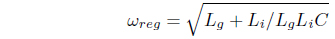
is the resonance frequency component.
In order to analyze the effect of the resonance frequency component on the grid current, the transfer function between the converter voltage and the grid current can be expressed as follows, ignoring the resistance component:

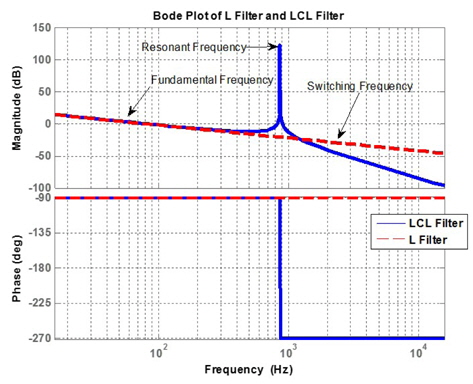
Figure 2 shows a 2.0-mH L filter, 1.0 mH, 22.5 uF, 1.0 mH and the Bode plot of the LCL filter in equation (3), which shows an excellent screening performance of the LCL filter. but it is possible to confirm that the resonance frequency component reveals. Because of the resonance frequency component, the total harmonic distortion (THD) becomes worse. This causes a low PF on the grid side since the reactive current is input to the filter capacitor.
3. FL-SMC Resonant Control with Observer
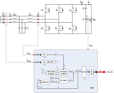
Figure 3 is a control block diagram of control method of an observer-based FL-SMC. In equation (1), the current controller can be designed as a type of PI controller by using the differential equation of the converter current.

Herein, the controller for reducing the resonance frequency component is designed by using the differential equation of the grid current of equation (1). At this point, by combining feedback linearization with a sliding mode control, nonlinearity is reduced and quick control response is achieved.
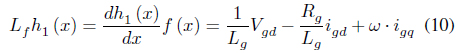
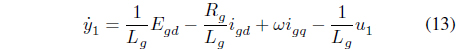
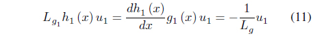
Feedback linearization is a technique that reduces the nonlinearity of nonlinear systems, in which an equivalent model including nonlinearity can be switched to a linear model [11]. In order to design a controller that reduces the resonance frequency component, in the differential equation of equation (1), when the differential equation of the grid current is expressed as a state equation like equation (4), it is to be equation (5).

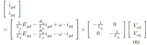
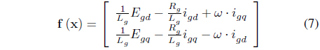

Here it is possible to define the state variables as , the output as , and the control input as .
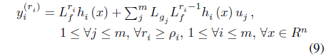
The input-output feedback linearization is applied using equation (9). The differentiation is repeatedly applied to the output until the input is revealed, and the number of differentiations is called the relative degree. For example, the relative degree of equation (6) is 1 because the input of the equation is revealed by one differentiation.
Herein,
When the differential on the first output is organized considering the relative degree, it is as follows:


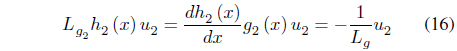
When the differential on the second output is organized considering the relative degree, it is as follows:
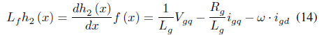

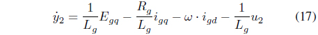
Using equations (14) and (17), when the linearized state equation is to be written again, it is as follows:

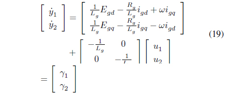
When equation (19) is organized about the control input:
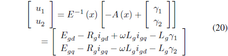
When equation (20) is rewritten by substituting the input of the state equation, the linearized state equation can be obtained, and
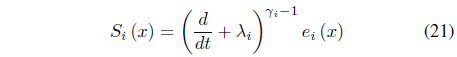
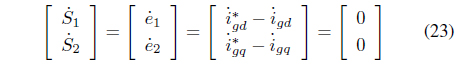
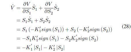
A sliding mode surface is composed of an equation that satisfies

Herein,
Since the relative degree is 1, the sliding surface can be defined as follows:

In order to converge an error value to the sliding surface in the sliding mode control, equation (23) should be satisfied:

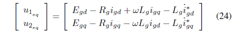
When substituting the differential equation on grid current into equation (23), it is possible to determine the control input of equation (20) and the control input of the equivalence.

The control rules of the sliding mode control can be defined as follows:

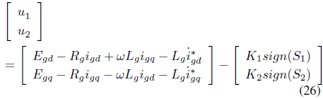
The control input of the controller that reduces the resonance frequency component can be defined as follows:
The grid-side
3.3 Stability Determination of Controller
The stability of the controller is determined by using a Lyapunov function. A Lyapunov function candidate is defined as follows:

When the partial derivative from the Lyapunov function candidate regarding

It is asymptotically stable since is always .
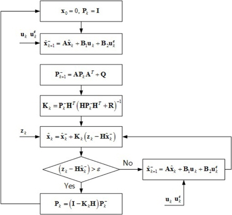
3.4 Recursive Suboptimum Observer
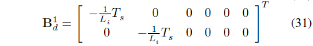
In order to estimate the grid current, the observer is designed by using an extended Kalman filter. The state equation is determined by using the differential equation of equation (1), to which discretization is applied as follows. At this point, the grid voltage is assumed as a disturbance.

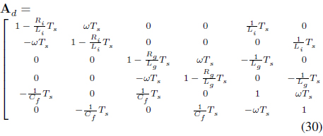


wherein the control variable, disturbance, state variable, output variable are as follows:


The extended Kalman filter is largely divided into two process. In the first process, time update, the prediction value is calculated by using equation (29). The error covariance is predicted by using equation (39):

In the second process, measurement update, the Kalman gain is calculated by equation (40) in advance:

wherein R is the covariance matrix of the measurement noise.
Next, in order to correct the errors of the prediction value, the estimated value is determined by using the observed value and the error of the prediction value, as shown in equation (41).

wherein is the state estimation value, and is the state prediction value.
By using equation (42), the covariance matrix is calculated. It is used to the next covariance matrix prediction value.

By repeatedly carrying out (42) in equation >(39), the Kalman gain is calculated in such a way that the error covariance becomes small.
The error covariance matrix is converged to a consistent value, with the Kalman gain also being a consistent value. At this time, the converged error covariance matrix is determined by seeking the value of an algebraic Riccati equation, while the Kalman gain can be earned by using the converged error covariance matrix. However, it is difficult to derive the value of the algebraic Riccati equation. Thus, if the error between the measurement value and the state observed variables is calculated, entering the range of allowable error, and the error covariance doesn’t get to be calculated with estimating as Kalman gain of normal state.

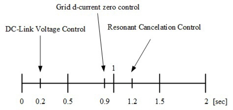
In order to confirm the performance of the proposed controller and the observer, a simulation is conducted using PSIM 9.0. The system parameters used in the simulation are listed in Table 1. The scenario of the simulation, as shown in Figure 5, first sets the DC-link voltage control at 0.2 s, the PF control of the grid side at 0.9 s, and the resonance control at 1.2 s.
[Table 1.] Simulation and Experimental System Parameters
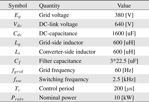
Simulation and Experimental System Parameters
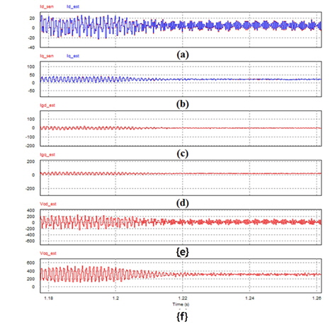
Figure 6 shows the waveform comparing the observed state variables with the actual measured values. Regarding the measured variables, which are observed with few errors, all state variables are observed.
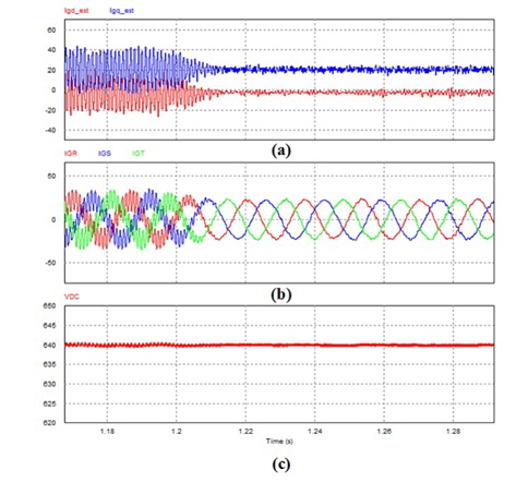
Figure 7 shows the converter-side
This paper proposes an active damping control method for a grid-side converter with an LCL grid filter in the back-to-back converter. Generally, a power converter measures the current of the converter side for current control. Because the power converter controls the reactive current of the grid side to zero, the reactive current is input to the capacitor of the filter on the grid side. Because the power factor of the grid side worsens, the power quality also worsens due to the resonance frequency component of the LCL filter. This paper proposed a method to enhance the efficiency of the system and the power quality by accomplishing the following: control the PF of the grid side to ±1 by applying a grid current observer by using a recursive suboptimum observer, and remove the resonance frequency component of the LCL filter by using a resonant controller. The performance of the proposed observer is verified by confirming the errors between the measured current waveform and the observed current waveform. This is done by installing a current sensor on the grid side. In addition, it is confirmed that the FL-SMC resonant controller removes the resonant frequency component by analyzing the frequency of the grid current. The active power filter that removes not only the LCL filter resonance frequency, but also the generating harmonics at the grid requires additional study. Future research is expected to focus on these topics.