It is well documented that over the last two decades an increasing and worldwide expansion of the international production network has been achieved (e.g. Kimura, 2006; Arndt & Kierzkowski, 2001). Outsourcing activities, vertical multinationals, and international trade in parts and components constitute different aspects of this phenomenon. This new wave of deepening global economic integration has led to the emergence of a new type of international specialization patterns among countries, labeled in the literature as vertical specialization.
There is by now accumulated evidence showing that vertical-specialization based trade has risen much faster than conventional exchanges of final goods, and is currently dominating world trade (Bridgman, 2010; Amador & Cabral, 2009; Breda
In East Asia, fragmentation in electronics is especially pronounced and developed. In this region large intra- and extra-regional production sharing networks have been formed and expanded (Hiratsuka, 2008; Kimura
Given the rising importance of the subject, there is a large and expanding literature on the trends, patterns, and determinants of vertical specialization (e.g. Miroudot & Ragoussis, 2009; Li, 2009; Dean
However, less attention has been given to the role and quantitative effect of a country’s extent of vertical specialization and participation in production networks on the country’s export performance. Given the increasing importance of global production sharing in electronics, empirical analyses on the export determinants at the country level should take into account and control for the extent of international fragmentation. Particularly for the case of the East Asian region and the electronics sector, it is often claimed that international trade and specialization patterns must be understood in the context of production fragmentation (e.g. Ando and Kimura, 2009; Haddad, 2007).
Nonetheless, the question of how fragmentation affects a country’s export development and performance has not been addressed explicitly. One exception, for instance, is Bonham
There are also some studies on the implications of fragmentation for an economy’s exports that take a country-specific view. Without providing a formal explanatory analysis, Kimura and Obashi (2008) examine this issue for China using regional data. They claim that the observed differences in export performance in electronics and machinery products across Chinese regions is partly explained by the cross-regional differences in the extent of participation in the East Asian production networks. Cieslik (2009) assesses empirically the role and impact of production sharing between Poland and the OECD countries on Poland’s trade volume with the OECD. It is found that, together with other country-level determinants, vertical production networks, as proxied by FDI, explain Poland’s trade with its trading partners.1
Two recent studies using large German establishment datasets investigate the effects of production fragmentation on a firm’s exports and other measures of firm performance (Moser
It has to be noted that the above empirical papers investigating to some extent this issue directly or indirectly have several limitations. The proxy for fragmentation that some studies use, such as FDI flows (Bonham
Furthermore, even vertical FDI does not fully capture a country’s extent of production sharing, as fragmentation can take place between independent firms (through arm’s length transactions) and not only within multinationals. The empirical analysis in some cases is not explicitly based on a relevant theoretical model and the regression equation is rather ad hoc (Moser
Therefore, to assess rigorously the impact of fragmentation on electronics exports at the country-level, this paper applies an empirical framework specifically for this purpose. This framework includes a measure of fragmentation that corresponds to the theoretical concept of fragmentation and VS, as measured by a relative VS index, suitable for cross-country analyses. As the phenomenon of VS is correctly and fully captured in our empirical analysis, its impact can be evaluated with greater precision, reliability, and confidence.
In addition, the comprehensive dataset that has been created and utilized for our panel-econometric analysis covers the 2000–2008 period and includes 28 developed and developing countries,which account for over97%ofworld ICT exports. This enables us to examine the effect of global fragmentation during a recent time periodwhere vertical production networks have been expanding in size and scope. The empirical analysis also allows the assessment of the dynamics with respect to fragmentation and export development.
The rest of the paper is structured as follows. Section 2 reviews the conceptual and theoretical background of international production fragmentation and vertical specialization. Section 3 examines the patterns and dynamics of electronics exports and vertical specialization across our sample of countries. Additionally, the co-movement and relationship between these two variables is also investigated through a first simple correlation analysis. Section 4 presents the empirical modeling framework and assesses the role, quantitative impact, and relative importance of vertical specialization on a country’s export performance in electronics goods. Finally, section 5 presents some concluding remarks and policy implications.
1Although the author provides an interpretation of the findings that give less support for a vertical FDI scenario, the theoretically derived estimable equation as well as the estimated coefficients of the FDI variable and some additional explanatory variables related to factor proportions and Heckscher-Ohlin specialization, which are all relevant also in the case of production sharing, hint at the relevance and significance of international production sharing for oland’s trade with the OECD.
2. Conceptual and Theoretical Background
International production fragmentation can be described as the phenomenon in which the production of a final good is fragmented or sliced into several production stages, which take place in different countries. The various intermediate goods, resulting from each production stage at a different location, are combined in the last stage to produce the final good. International trade in intermediate inputs plays a crucial role here, as it is an integral part of the overall production process. It constitutes a service link connecting all separate production blocks.
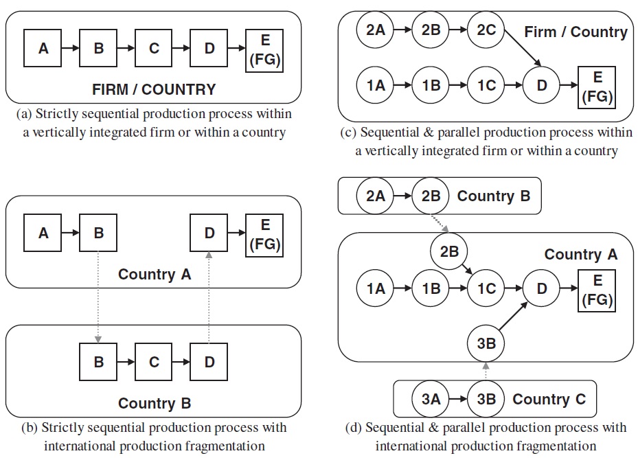
Figure 1 illustrates graphically the concept of international production fragmentation in the case of both a strictly sequential and a parallel-sequential production process of a manufacturing good. Panel (a) of the figure shows the case of a strictly sequential production process that takes place within a vertically integrated firm (where all stages are carried out) or within a country (the firm acquires some of the intermediate production stages only from local suppliers). In this strictly sequential process some initial raw materials (block A) are being transformed progressively through various stages into processed intermediate goods (blocks B, C, and D) and finally into the final good (final production stage E).
As shown in panel (b), with international production fragmentation, only a subset of the sequential production stages are being carried out in the home country (A), while the remaining blocks are produced in another country (B). In particular, in our simplified example with two countries, country A produces the good-in-process B, which is then exported to country B (grey dotted arrow) so that intermediate sequential production stages C and D are produced in that country. From there, production block D is exported to country A, where the final transformation occurs and the final consumer good is produced (stage E).
In reality, many production processes are not strictly sequential, but rather involve sequential as well as parallel processes. In this case, there is not a single sequential chain, but several parallel chains that are later combined to produce goods-in-process at a more advanced stage and the final good. This is illustrated in panels (c) and (d) of the figure. The number before the letter of the production block denotes the parallel chain. Thus, in the case of intra-country (or vertically integrated firm) production, we start with parallel production chains 1 and 2, which result in intermediate goods 1C and 2C. These intermediate stages are combined to produce stageDfromwhich the final transformation occurs. Finally, in panel (d), international production fragmentation is shown for a production process with three parallel-sequential chains and three countries.
Global outsourcing and vertical specialization constitute prominent characteristics and features of this production fragmentation process. It has, however, to be noted that these concepts, although related, are not synonymous. As Hummels
Onthe other hand, according to the conceptual definitions of the above authors, the more general case of outsourcing involves a one-way intermediate goods trade among countries, where the imported intermediates are used only for the production and subsequent consumption of the resulting final good within the country. This final good is not exported nor are the imported intermediate goods used to produce other intermediate inputs (goods-in-process) to be exported, as in the case of vertical specialization.
Although Figure 1 illustrates the concept of international production fragmentation, it provides no information on the economic rationale and motivation behind this process. Given that countries differ in factor productivities and relative factor endowments, the driving forces behind such production fragmentation may be found in the different labor skills and in the different factor proportions that different production stages require.
If the fragments exhibit differences in labor requirements, the different production stages are carried out and located in countries inwhich the skills of their labor force match the labor skills requirements of those particular segments. This fragmentation pattern across countries with different labor productivities and skills generates Ricardian specialization patterns and gains from trade. Additionally, if the segments exhibit differences in factor proportion requirements, the various production blocks locate in countries in which their relative factor abundances match the factor-intensities of those particular fragments. The resulting international production fragmentation pattern creates a Heckscher-Ohlin (H-O) type of specialization across countries. Thus, the more labor-intensive production stages locate in labor-abundant economies and the more capital intensive fragments locate in capital-abundant economies.
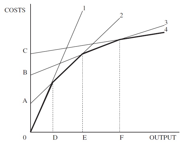
By taking advantage of the cross-country dissimilarities in factor skills and prices, international production fragmentation reduces significantly the production cost in each segment and the overall production cost of the final good. This is illustrated more clearly in Figure 2, which shows production costs as a function of the output level. Line segment 1 depicts the cost curve when all the production process is carried out within a vertically integrated firm or within a country (as shown in panels (a) and (c) of Figure 1) with constant returns to scale.
The other line segments refer to the cost functions for a progressively fragmented production process, which are also subject to constant returns to scale. Thus, line segment 2 illustrates the case where the production process is fragmented between two countries (some stages are carried out in one country and some other stages in the other country). This results in a reduction in marginal production costs as indicated by the smaller slope of line segment 2. Since these production blocks among the two countries have to be coordinated and transported fromone country to the other (in order for the overall production process to be completed) there is an international coordination cost associated with this fragmentation. This cost of service links is represented in the figure by the distance 0A and the fragmentation pattern 2 is cost-effective for output level greater than 0D.
Similarly, line segments 3 and 4 represent cost curves for a progressively finer fragmentation pattern. Here, several production stages are located among several countries and marginal costs are further reduced by matching even better the production requirements of the segments to the country differences. Hence, cost curve 4 represents the most fragmented production pattern in the figure, in which the marginal cost (slope) is lowest and the coordination cost is 0C (the highest). The bold locus depicts the fragmented production pattern that minimizes total production costs. As it can be seen from the figure, international production fragmentation leads to increasing returns to scale.
Theoretical analyses on the phenomena of trade in intermediate products and production fragmentation date back to the 1980s and 1990s (e.g. Sanyal & Jones, 1982; Jones & Kierzkowski, 1990) and have since been extended and examined further with an increasing interest (e.g. Arndt & Kierzkowski, 2001; Deardorff, 2001; Grossman & Helpman, 2002; Yi, 2003; Kimura & Ando, 2005; Luthje, 2005, 2006; Markusen & Venables, 2007; Baldwin & Robert-Nicoud, 2010).
Although this line of research investigates and provides insights in a number of issues, we limit our attention on the implications with regard to export patterns, and more precisely on export performance. First, the effects of international production fragmentation have been examined with diagrammatic analyses within a rather simple modeling context. For instance, taking an HO view with two countries and two goods (where one good is fragmented), Arndt’s (2001) examination reveals that fragmentation within a free trade area leads both countries to produce and export different intermediates (production stages) of the fragmented good.
Additionally, both countries continue to produce the final good with the fragmented technology (imported intermediate goods), and the bilateral trade occurs in the components of the fragmented good. The output of this final good in both countries increases due to lower overall production costs and increased productivity, as does the export volume. An implication is that their exports of the fragmented good could also rise towards third countries, as they produce with lower costs compared with countries that do not use the fragmented production process.
This can also be extrapolated from Figure 2, where it is evident that firms (and in a macroeconomic extension, countries with such firms) that make use of an internationally fragmented production technology exhibit decreasing marginal costs and experience an increase in the output level. This feature makes them more cost competitive compared to non-fragmented firms, and thus their export performance may improve significantly.
In a similar theoretical exercise, Deardorff (2001) examines the issue with both a graphical and a formal mathematical analysis within a Ricardian as well as HO setting. Depending on how and whether fragmentation changes the prices, a country could also specialize completely in the intermediate good and export it, with the other country specializing in the final good. In addition, both countries would experience an increase in their output level.
In more formal and general equilibrium analyses, where fragmentation is allowed to occur in any sector and direction, typically a variety of results can be generated and the outcomes are rather ambiguous (depending on certain conditions) than straightforward predictions.Without going into the details, in Baldwin and Robert-Nicoud (2010), for instance, international production fragmentation can lead the home country that outsources the given tasks to experience a significant increase in the output in both goods. Production in the foreign country increases also at least in one sector and typically intra-industry trade occurs (Home exports the final goods and Foreign exports the fragments as well as some quantity of final goods).
Additionally, output may rise further in the foreign country with the possibility of two-way intra-industry outsourcing. Thus, although the results are not clearcut, a typical scenario is that the countries engaging in international production sharing should be expected to experience cost savings and expansion in output and exports. Finally, in a multi-country approach within an HO framework, Markusen and Venables (2007) examine explicitly the effects of international fragmentation on trade volume. Their numerical results show that fragmentation leads to an export expansion in countries that engage in export activities, where the specialization can occur in the assembly activity or in the components of the fragmented product.
2For a discussion on this issue see, for instance, Hummels et al. (2001) or Chen et al. (2005).
3. Electronics Exports and Vertical Specialization across Countries
3.1 Patterns and Trends in Export Performance
In our empirical analysis we use data on electronics exports from theWTO international trade database. Electronics exports are defined as exports belonging in the following SITC (Standard International Trade Classification) categories: 75, 76, and 776 (office machines and automatic data processing machines; telecommunications and sound recording and reproducing apparatus and equipment; thermionic, cold cathode or photo-cathode valves and tubes). The data on electronics exports (as well as on total exports) for all countries in our sample are in US dollars at current prices and refer to a country’s world exports.
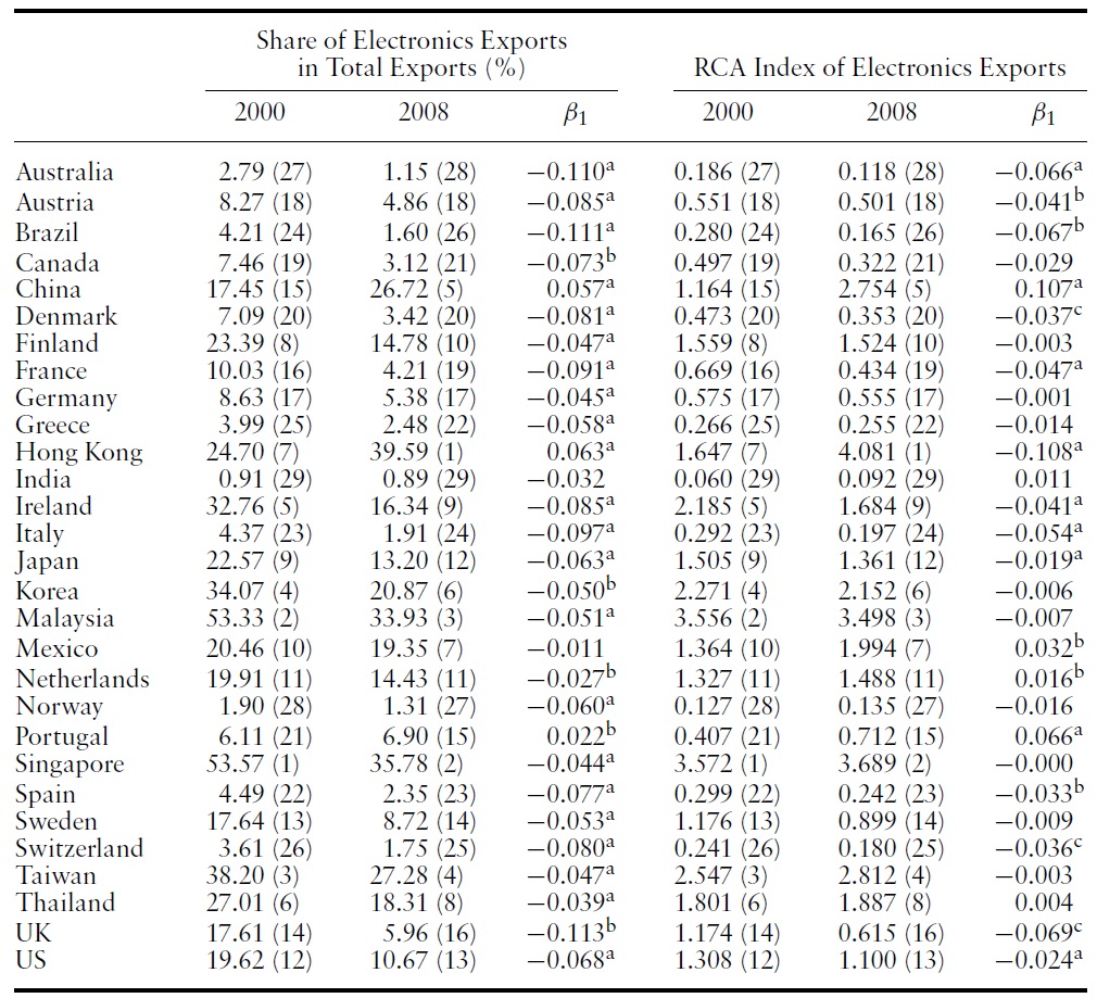
Table 1 shows the development in the share of electronics exports in total exports as well as in the Revealed Comparative Advantage (RCA) index between 2000 and 2008 for 29 countries. First, it is evident that some South-east Asian economies (e.g. Singapore, Malaysia, Taiwan, and Korea) and some smaller countries (such as Ireland and Finland) show the highest exports shares, indicating an especially high export concentration. These economies have RCA indices well above unity, revealing a strong export performance in the given product group relative to the world. Some advanced OECD economies (such as Japan, Netherlands, the US, Sweden, and the UK) show also high export shares in electronics goods.
[Table 1.] Export performance in electronics of 29 countries, 2000?2008

Export performance in electronics of 29 countries, 2000?2008
Secondly and more interestingly, there seems to be a negative trend in most countries. The exceptions are China, Hong-Kong, and Portugal. Although the table does not show all data (time) points, it reports the annual average growth rate, which has been estimated with a linear trend model. It is a general finding that a statistical significant negative trend is present, except in the aforementioned countries, which exhibit a significant positive trend. It has to be noted that a closer examination of the data shows that electronics exports are increasing in almost all countries in absolute terms, but due to the higher export growth rates in the other product groups, electronics exports in total exports are falling.
Thus, the export level in electronics goods is not falling; rather there is a decreasing export specialization (in terms of both a country’s concentration of electronics exports in total exports and a country’s export specialization of electronics goods within the world economy as indicated by the RCA index). Most importantly, however, China and Hong-Kong seem to have increased substantially their export shares, in terms of export concentration as well as export specialization in the global economy. This is a result of the particularly strong export growth that has been achieved in those economies in recent years. On the other hand, several OECD economies have witnessed a significant fall in both of those measures (especially the UK and Ireland).
3.2 Trends in Vertical Specialization
3.2.1 The measurement of VS
For identifying the vertical specialization trends and patterns across our sample of countries, we use the VS index3 developed by Amador and Cabral (2009).4 We employ this index because, by construction, it is a relative measure, suitable for international comparisons and cross-country studies.5 In addition, VS data calculated with this index are available for our panel of countries.
This measure combines data from international trade statistics and Input-Output (IO) matrices.6 Amador and Cabral’s (2009) index is based on the following reasoning and two-step methodology. In terms of relative international product specialization, a high export share in a given product (
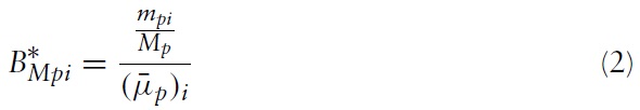
More specifically, the international product specialization index for exports as well as imports that is used for the calculation of the VS measure is a modified Balassa index, denoted
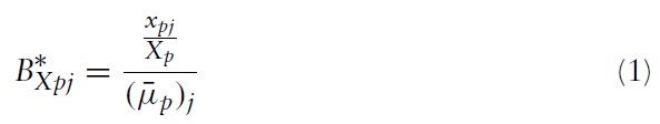

where
Amador and Cabral (2009) combine trade data at the ISIC 4-digit level for manufacturing goods (
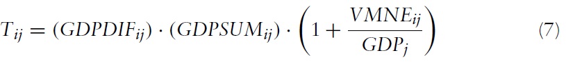
Thus, the first stage of the methodology is the identification of VS activities and is applied as follows. For every product pair (
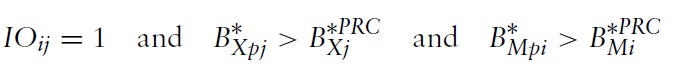
The above condition says that
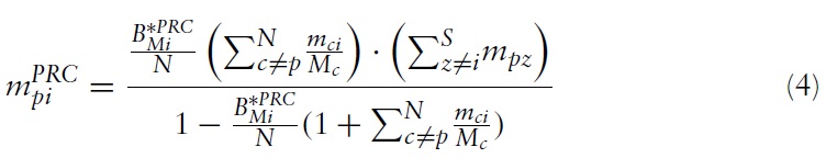
In the second stage,which involves the quantification of VS, in any given input

Solving equation (3) for

yields:

Equation (4) gives the value of the imported input

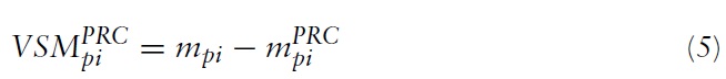
Now, the VS measure is computed as the value (amount) of the imported intermediate input

Since this calculation applies only for the cases that have been identified as VS from the first stage, the above equation takes only positive values. This measure, which reveals a country’s VS level (in value terms), can also be expressed as a percentage of a country’s total imports:

Equation (6) is the resulting VS index that reveals a country’s relative extent of VS (as a share of total imports). The VS measure can be calculated for individual sectors (product groups) and for different definitions of intermediate inputs. It has to be noted that VS shows the value of the intermediate goods imports (
3.2.2 The extent of VS
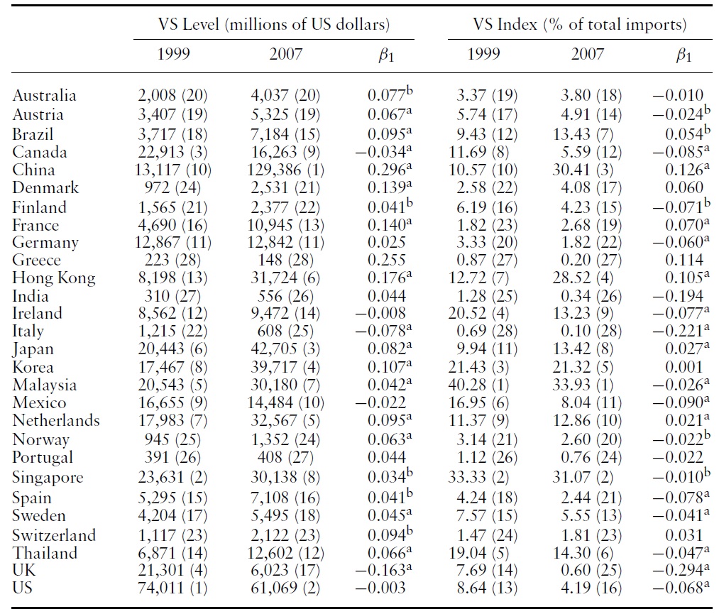
Table 2 reports the cross-country vertical specialization trends over the 1999– 2007 period. The table shows two VS measures: the first is the value of imported intermediates used in the country’s exports in levels (millions of US dollars) – equation (5) – and the second is this value expressed as a percentage of total imports – equation (6). In general, it seems that larger countries tend to exhibit higher VS levels than smaller countries. This is rather expected since a higher absolute value of intermediate imports will tend to be present in countries with a higher absolute value of exports; countries that tend to be the larger ones.
[Table 2.] Vertical specialization of 28 countries, 1999?2007

Vertical specialization of 28 countries, 1999?2007
However, there are some notable exceptions to this: Singapore and Malaysia rank especially high in the list, whilst Brazil and India show a low ranking. Additionally, France and Germany fall rather in a medium ranking range. In 1999, the US exhibits by far the highest VS level, whereas in 2007 the US has been overtaken by China in this respect and ranks in second place. China has witnessed an impressive growth in her vertical specialization level over 1999–2007 with an average annual growth rate of about 30%. In most countries, there seems to be a general upward trend in the VS level.
As regards vertical specialization trends in relative terms, it is evident that the South-east and East Asian countries included in our sample exhibit the highest VS indices. According to these results, in recent years vertical specialization is a phenomenon that is especially important in Malaysia, Singapore, and the two ‘Chinese economies’ (mainland and Hong-Kong). Two European countries (Ireland and the Netherlands) and two Latin-American countries (Brazil andMexico) also show a significant VS index. There are 15 statistically significant negative time trends in the VS share, indicating that there is to some extent a decreasing tendency in some countries.
From examining the two tables we have some indication that countries that exhibit a high share of electronics exports in total exports tend also to exhibit a high VS index. This could imply that there is a positive correlation between a country’s electronics export share and a country’s extent of VS in relative terms. Accordingly, we would expect that highly vertically specialized countries exhibit a higher export share in electronics goods, while countries with a low VS share show a lower export share.
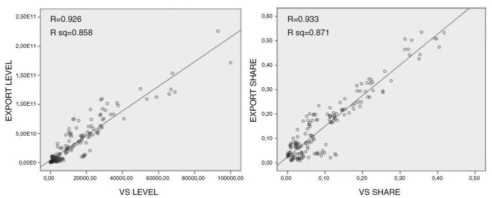
In order to examine this issue we conduct two correlation analyses. In the first analysis, the correlation between the export level in electronics goods and the VS level is examined (both in value, thus in absolute terms). The second analysis involves the examination of the correlation between the electronics export share in total exports and the VS share. Figure 3 shows the results of the two correlation analyses, which both produce highly statistically significant Pearson correlation coefficients. From the left panel of the figure we can see that there is a very strong linear correlation between the value of electronics exports and the value of the imported intermediates embodied in a country’s exports (VS level) with a correlation coefficient of 0.926.
Additionally, it can be seen from the figure that a linear regression line has been fitted, and thus a simple regression analysis has been also conducted with exports as the dependent variable.The coefficient of determination for this simple regression is also very high, 0.858, indicating that about 86% of the cross-country variance in the export level can be explained by the variability in the VS level. In the right panel of the figure the correlation (and simple regression) analysis for the electronics export share and the VS index is shown. It is apparent that there is an extremely high correlation between export share and VS share. The correlation coefficient is 0.933 and the coefficient of determination of the fitted regression equation is 0.871.
Thus, the general picture emerging fromcross-examining the two tables regarding the relationship between the export share and VS index is confirmed by our correlation analysis. Furthermore, the analysis showed that there is also a positive correlation between the export level of electronics goods and the level of vertical specialization (in value terms).
3Since we are concerned with electronics exports, we use their VS measure which corresponds to the electronics sector and is calculated from 33 components and parts. Those components are intermediate inputs mostly of electronics and machinery products. 4The data on vertical specialization for the countries in our sample have been kindly provided by Amador and Cabral (2009) upon request by the author. 5For an overview of different measures and indices related to the phenomena of international production fragmentation and vertical specialization see, for instance, Molnar et al. (2007) and Formentini and Iapadre (2008). 6The information from the IO tables is necessary for the identification of the production chain (i.e. whether a good is an intermediate good input used in the production of another good). The information from the trade statistics is needed for the identification and measurement of VS. 7Notably, this identification is dependent upon an arbitrarily VS threshold (the PRC). Furthermore, high values of both B∗ indices (for exports and imports) may be due to horizontal intra-industry trade or other country-specific characteristics that would explain a country’s trade shares to be higher than the corresponding world average. Since the PRC threshold is particularly crucial for this procedure, several high threshold levels have been chosen.
4. VS and Export Performance: Panel Econometric Analysis
Although a correlation as well as simple regression analysis can be informative on the co-movement and linear relationship between the underlying variables, they are both restrictive and cannot provide the information our examination requires. In this section,we examine with a panel-econometric model the effect of a country’s extent of vertical specialization and participation in the international production fragmentation on its export performance in electronics.
Before outlining our modeling framework, it could be pointed out that a general insight of the theories on international fragmentation, presented in section 2, is that output and exports are generally expected to increase in countries engaged in fragmentation. Hence, VS is potentially a significant determinant of a country’s exports, and thus we could simply include and test it in a parsimonious empirical export model.8 However, we will proceed and examine this issue by means of a more structural approach, where the estimating regression equation is related and derived from a theoretical model.
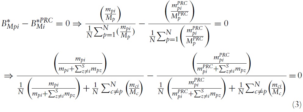
A particularly relevant theoretical framework for our empirical analysis is the reformulated and extended Chamberlin-Heckscher-Ohlin (C-H-O) model with multinational firms and production fragmentation (Helpman & Krugman, 1987; Markusen, 2004). Without going into the details, a trade volume equation can be derived from the C-H-O model, which basically predicts that bilateral trade volume depends positively on bilateral economic similarity (GDPDIF), joint economic size (GDPSUM), and bilateral production sharing activities:
where
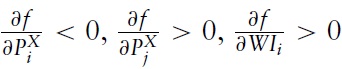
Thus, for our empirical analysis, we apply an analytical framework of international trade that allows the use of aggregated trade data in the empirical implementation (world exports of the countries in our sample aswell as an overall measure of a country’s fragmentation). More specifically, we base our analysis on Goldstein and Khan’s (1978, 1985) imperfect substitutes model, where domestic and foreign goods are not perfect substitutes and each country can at the same time be an exporter and an importer of a given traded good. The imperfect substitution assumption is particularly relevant in the case of differentiated manufacturing products such as electronics. This model is based on conventional consumer choice and production theory, where consumers and producers maximize utility and profits, respectively. It is represented as a system of simultaneous equations of export demand and export supply that simultaneously determine the export quantity and export price:
with


with
where

is world export demand of country

is the export price of

is the export price of country

is world export supply of
Besides the above discussion and that of section 2, the rationale of VS to be included in the model can be justified also from the modified C-H-O model, as described by equation (7). In this case if, for instance, two countries have similar economic size and the same trade partners, but differ in the extent of production sharing with those partners, then the country with the higher VS will exhibit a higher overall trade volume (world trade) compared with the country with less involvement in production fragmentation.
A simple estimable version of the simultaneous equations system can usually take the following form:


where RER is the real effective exchange rate in country


where
The reduced-formsingle export equation (12) serves as the basis of our regression model and in a second stage it is augmented with additional explanatory variables that are potentially important export determinants in electronics goods.
4.2 Econometric Specification and Methodology
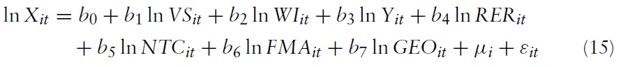
The baseline specification of our econometric model of cross-country export performance is represented by the following log-linear panel regression equation:


where
We are specifically interested in the estimated parameter
To test for robustness with regard to the impact of VS, an extended model is also estimated, in which several additional control variables are included. In this augmented model specification the additional regressors relate to supply-side factors, and thus would be included in the export supply equation (11), as well as to market or demand-side factors that would be included in equation (10). More specifically, the model is extended by including explanatory variables such as national technological capability and productivity (NTC), foreign market access (FMA), and internal geography (GEO).
Although, with fragmentation, the overall production process of electronics goods cannot be considered as technology-intensive, technology-related factors may still be relevant to some extent. An improved technological capability and production structure would be associated with increased productivity, resulting in Ricardian comparative advantage. This implies that technology-related factors may not only be relevant for certain knowledge and innovation-intensive segments. Rather, technology may have a more general positive effect on a country’s productivity regardless in which particular segment it specializes, and hence on a country’s international competitiveness and export performance.
Thus, our technology variable corresponds more to the notion of a country’s technological and productive capabilities (Lall, 1992), which reflect technological advancements in the production organization, which raise productivity levels. According to Lall (1992) those capabilities are mainly determined by the country’s technological effort and investment in physical and human capital.
The remaining two control variables to be included in the augmented model relate to economic geography factors. Those factors are particularly stressed by recent advances in the theoretical and empirical literature on geography and trade. More specifically, Redding and Venables (2002) develop a theoretical model of cross-country export performance and derive from it an empirical log-linear export equation. According to their model, export performance is explained by the exporting country’s supply capacity, FMA (reflecting external geography), internal geography, and comparative cost of exporting (reflecting comparative cost advantage).
Notably, our baseline export equation resembles (to some extent) the specification of Redding and Venables (2002), where supply capacity and comparative cost advantage (proxied here by RER) are also included. Furthermore, our model becomes even more similar with the addition of the two economic geography variables (FMA and GEO).
The FMA variable, which is related to the notion of market potential of Harris (1954), reveals a country’s extent of access to international markets, taking into account the relative geographical position and trade costs of an exporting country to the foreign markets. A good market potential or access within a region (here the world economy) shows that an exporting country is geographically close to (and/or exhibits low trade costs with) major consumption markets (within the world economy), and thus is expected to have a positive impact on the country’s export performance.
Lastly, the costs associated with getting the goods that are produced in exporting country
Thus, the augmented model is represented by the following equation:
where

and where
The inclusion of the country-specific effects is particularly important in order to control for omitted variables bias as well as to account for unobserved individual heterogeneity. Hausman tests are conducted in order to reveal the appropriate panel specification (fixed or random effects). The null hypothesis of the Hausman test that the individual specific effects are uncorrelated with the regressors is clearly rejected in both regressions. Thus, the models are estimated with the fixed-effects panel estimator. Additionally, panel robust-standard errors are used to correct for heteroskedasticity, and the residuals are adjusted to followan AR(1) process in order to control for the presence of first-order serial correlation:

where |
Besides the above issues and corrections regarding our panel-econometric estimation, we have also to take into account the potential endogeneity problem associated with the
Therefore we conduct Durbin-Wu-Hausman endogeneity tests for both VS measures (used in the two models in level and share form) in order to check for the exogeneity of our main explanatory variable of interest. In the panel fixedeffects model the consistency of the estimation results with respect to the VS variable and the other regressors rests on the assumption of exogeneity. In case of an endogeneity problem, the appropriate estimation method for our model is panel instrumental variables (IV) estimation. In order to perform this test we have to estimate the Panel IV as well as standard fixed-effects models.We have to choose suitable instrumental variables for our suspected endogenous VS variable to estimate the panel IV (2 stage least squares) model. The instruments have to be sufficiently correlated with the instrumented (endogenous) variable and at the same time uncorrelated with the error term of the second-stage regression.
We base the choice for the appropriate instruments on trade theory. In particular, as already discussed in section 2, the motivation for vertical specialization (production fragmentation) is found in the different labor skills and factor proportions requirements of different fragments. Consequently, the larger the differences in labor skills-productivities and relative factor endowments between a country and its trade partners, the larger the economic rationale for (and gains from) vertical specialization.
This, in turn, implies that the overall extent of VS will be higher for a country with such large skill and endowment differences. Thus, the two comparative advantage related instrumental variables that influence a country’s extent of vertical specialization are a country’s overall extent of differences in labor skills-productivities and relative factor endowments with its trade partners.
Besides the above two variables, we include a third instrument, which from a theoretical as well as empirical point of view is very important with regard to production fragmentation. This variable is the cost of the service links that are required for the connection of the different production segments produced in different countries. These service link or coordination costs have a negative impact on the degree of fragmentation. Consequently, countries where the coordination costs are high are expected to be less involved in international production fragmentation, whilst countries with low service link costs and advanced logistics infrastructure are expected to be relatively more engaged in fragmentation activities.
Jones
The endogeneity tests reveal that the VS variable in both models (in level and share form) is endogenous and thus panel IV estimation is required. As we have data for all variables except for VS for the year 2008, we estimate also the two models for the 2000–2008 period by including a time-lagged VS variable (
4.3 Variables and Dataset Construction
As already mentioned, the export data for the two dependent variables are taken from the WTO international trade statistics database, and the two VS measures, as given by equations (5) and (6), come from Amador and Cabral (2009).
The world income (demand) variable (WI) for country’s
This measure varies across our sample of exporting countries rather than being the same for all
In our model, the productive capacity (
As the data for the combinedVAin ISIC sectors 30, 31, and 32 are only available for a small number of countries in our sample, the VA in machinery and transport equipment (MTVA), for which we have data for more countries, is chosen as the relevant electronics measure for the correlation analysis.11 We find that there is a highly statistically significant and strong correlation between MVA and MTVA (
The real effective exchange rate (RER) variable is expressed as an index, where the base year is 2005.The price deflator used for the calculation of the real effective exchange rate is the consumer price index (CPI). A fall or depreciation of the RER variable indicates an improvement of a country’s international competitiveness, whereas an increase indicates the opposite. The data source for most countries in our sample is the IMF’s International Financial Statistics (IFS) database, except for Brazil (which is Banco Central do Brasil), Hong Kong (Hong-Kong Monetary Authority), India (Reserve Bank of India), Korea, and Mexico (both OECD. Stat database), and Thailand (Bank of Thailand). Where necessary, the RER indices have been re-indexed to the year 2005, so that for all countries we have the same base year.
Our national technological capability and productivity (NTC) variable is a composite of three factors that determine a country’sNTC. As already discussed, Lall (1992) identifies technological effort and innovation, physical capital accumulation, and investment in human capital as the three main factors for a country’s success with respect to NTC.We proxy technological effort, physical capital, and human capital by the research and development (R & D) expenditure, the gross fixed capital formation (GFCF), and the public spending on education (PSE), respectively (all in US dollars).12 The final resulting NTC variable is calculated as a weighted average with the following weights: R & D (0.5), GFCF (0.2), PSE (0.3). These particular proxies have also been chosen because they are available for all countries in our sample. The data are obtained from the WDI database except for China’s PSE which is taken from Barnett and Brooks (2010).
A country’s foreign market access (FMA) in our case has to reflect this access specifically with respect to international markets for electronics goods. Thus, general expenditure (such as GDP) is not appropriate to be used as the relevant expenditure measure, indicating the market size of the partner countries. The consumption market size should relate to electronics goods, and therefore we take the ICT expenditure within a country as our relevant measure. The FMA for each exporting country
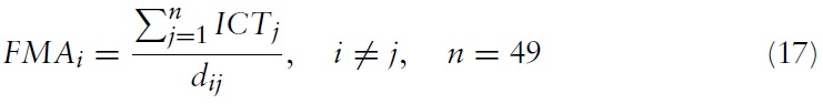
where
Our last explanatory variable internal geography (GEO) is calculated as a composite of three variables: road density (DEN), telephone lines per 100 people (TEL), and percentage of the population living within 100 kilometers of the coast (POP). Redding and Venables (2002) use only POP to proxy GEO in their crosssection analysis. Since POP is only available for a reference year,we cannot use it in our panel-econometric analysis as it is time-invariant. Therefore, we construct a more comprehensive GEO variable, where internal transport cost is also reflected by DEN and TEL.
These infrastructure-related variables certainly have an effect on a country’s internal geography. We assume that POP does not change over our time period and calculate the GEO as a weighted average with the following weights: DEN (0.25), TEL (0.25), POP (0.5).DENand TEL are obtained from the WDI database and POP is taken from the Compendium of Environmental Sustainability Indicator Collections, Socioeconomic Data and Applications Center, Center for International Earth Science Information Network, Columbia University.
Regarding our instrumental variables, the labor skill-productivity is proxied by the country’s labor cost in the manufacturing sector and the relative factor endowments by the capital-labor ratio. Here, capital is measured by the gross fixed capital formation and labor by the country’s labor force. For the calculation of the overall extent of a country’s differences in those two variables, we first calculate the bilateral differences between the 28 exporting countries in our regression sample with 35 partner countries. The final measure for both variables is a tradeweighted average of the bilateral differences. For the construction of those two variables we have used data from the labor statistics database (LABORSTA) of the International Labor Organization and the WDI database of theWorld Bank. Additionally, the bilateral trade data required for the calculation of the final overall measure come from the UN COMTRADE database.
Our third instrument, service link and coordination costs, is proxied by the average cost to export and import (US dollars per container) divided by the logistics performance index (LPI). Instead of using the overall LPI, we use the LPI index in the category ‘quality of trade and transport-related infrastructure’. The separate data available for cost to export and cost to import (per container) are used to create an overall average measure of trade cost relevant for supply chain services and fragmentation activities.This cost affects adversely a country’s extent of vertical specialization.
The LPI takes a continuous value from zero to five, where a higher value indicates a higher quality. A country with a high LPI value is more likely to exhibit the skills and infrastructure with regard to the supply chain services required for production fragmentation. Consequently, the LPI correlates positively with a country’s degree of participation in vertical production networks.This is reflected in the overall measure of service link costs, in which costs and quality are both taken into account.14 Since the LPI is the denominator in our constructed variable, a higher quality (LPI) makes the overall service link cost measure smaller.
In principle, we could just use the LPI to proxy for this instrument. However, the LPI is only available for one year, and therefore we construct the measure in the above-described way. We assume that the LPI is constant (does not change significantly) during our sample period and the time variation of the measure comes from the cost to export and import. Besides this data issue, the added benefit of having such a measure is that it takes into consideration both costs and quality. The required data are obtained from the WDI database.
For all the above-described variables, we construct a comprehensive and fully balanced panel dataset for 28 countries over the 2000–2008 period. This has been accomplished by obtaining data from various international databases and national sources and filling in the missing values by linear or polynomial interpolation techniques. The interpolation method used for any given variable has been based on the given data structure and the associated goodness of fit. An extrapolation technique similar to the above-described interpolation has been applied to our VS measure in order to extend the sample period for this variable. For reasons of precision and error minimization, this extension has been restricted to only two years (up to the year 2007).
We have eight sets of empirical results that are presented in Tables 3 through 6. More specifically, the first two tables refer to the panel IV models in level and share formfor both the basic as well as the extended specification. The remaining two tables pertain to the level and share models with the time-lagged VS variable and the extended sample period 2000–2008.
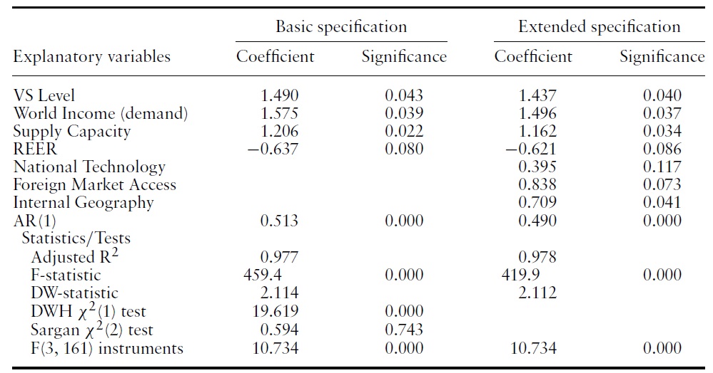
Turning first to the export level model for the 2000–2007 period (Table 3), it is apparent that the panel IV (2-stage least squares) model with the given instruments is indeed the appropriate estimation method. The null hypothesis of the Durbin-Wu-Hausman (DWH) endogeneity test that the VS-level variable is exogenous is rejected at the 1% level (with a
It is evident that vertical specialization has a strong and statistically significant effect on a country’s electronics export level. The export elasticity in the basic specification is about 1.5, indicating that a 1% increase in the VS level causes a 1.5% increase in a country’s ICT exports. All control variables show the expected coefficient signs and are statistically different from zero at various levels of significance. The world income-demand variable exerts the strongest influence on a country’s export level.The estimated income elasticity of demand for ICT exports is found to be close to 1.6. Supply capacity also exercises a rather strong effect on electronics exports with an elasticity of 1.2, whilst the impact of relative price competitiveness (REER) is much smaller.
These results are found to be robust in the extended specification, where the elasticities of the basic predictors show only a miniscule fall. The impact of a country’s VS level on electronics exports is still strong and statistically significant. As regards the additional regressors, foreign market access and internal geography exhibit rather high and significant elasticity coefficients, whereas the national technological capability and productivity variable is found to be insignificant.
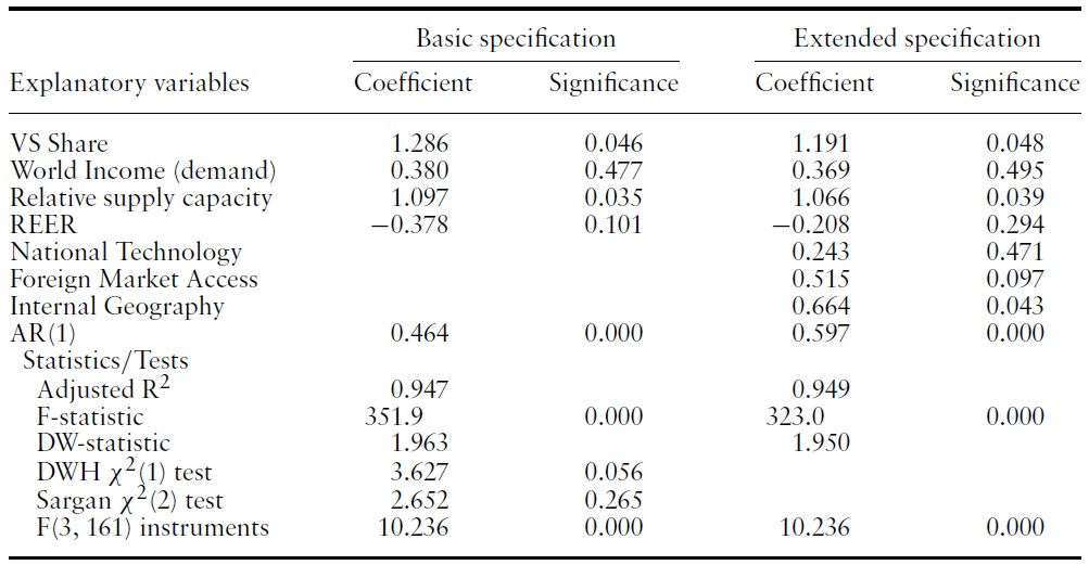
In the export share model, shown in Table 4, the panel IV estimator with country-specific fixed-effects is also found to be the correct panel-econometric method. The DWH endogeneity test rejects that the VS share variable is exogenous. However, in this case we can reject the null hypothesis only at slightly above the 5% level (
We find that a country’s VS share affects positively the country’s export share. The size of this effect is large, but not as large as in the export level model. The estimated elasticity suggests that a 1% rise in a country’s share of vertical specialization-based imports in total imports promotes an increase in the country’s share of electronics exports in total exports of about 1.3%. This effect is statistically significant at the 5% level and represents the strongest deterministic factor of a country’s relative ICT export performance within our model. With regard to the control variables, the world income-demand variable is found to exert no significant effect, suggesting that it does not constitute a determinant of a country’s export share in electronics. A country’s supply capacity, which here in the export share model is defined as the MVA to GDP ratio and therefore labeled as relative, has also a positive and significant elasticity.
The price competitiveness is found to be significant slightly above the 10% level with a rather low elasticity estimate. Overall, the model’s goodness of fit is pretty high, but lower compared with the export level model. The findings are robust, as in the extended specification, no significant changes occur with respect to our basic regressors, except for the REER variable, which becomes insignificant. The elasticity of the VS share variable drops slightly, but is still significant at the 5% level.Regarding the additional predictors, the internal geography variable appears to be the most significant with the strongest effect, whereas national technology is found to be statistically zero and FMA is only marginally significant at the 10% level.
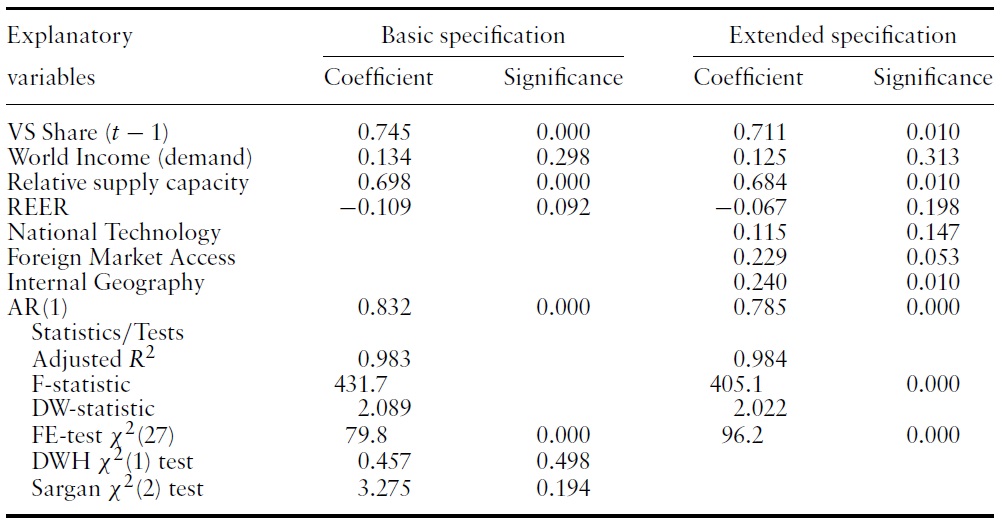
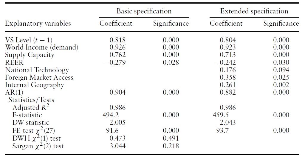
Table 5 reports the results for the fixed-effects export level model with the timelagged VS level variable, which is estimated for the period 2000 to 2008. Since the null hypothesis of theDWHendogeneity test that the time-laggedVS level variable is exogenous is not rejected, the model is estimated with the standard fixed-effects panel estimator. It is found that the time-lagged VS level variable exerts a strong and highly statistically significant effect on a country’s electronics exports. The coefficient estimate suggests that a 1% rise in the extent of a country’s vertical specialization raises ICT exports by 0.82%. The magnitude of this positive effect is, however, much smaller than the one found in the panel IV export level model.
The income elasticity of demand for electronics exports is found to be about 0.93. Thus, world income represents the relatively most important determinant of a country’s export performance. Supply capacity also determines positively the export level with an estimated elasticity of about 0.76, whilst relative price competitiveness has a statistically significant but rather low elasticity. These findings are robust in the extended specification. Although all three additional regressors are significant, the estimated coefficients indicate that their influence on a country’s ICT export level is rather weak.
Finally, the findings with regard to the impact of the time-lagged VS share on a country’s electronics export share are shown in Table 6. The VS share (
[Table 3.] Impact of VS level on electronics export level, Panel IV Model, 2000?2007

Impact of VS level on electronics export level, Panel IV Model, 2000?2007
From comparing and cross-examining all the above results, we firstly notice that the coefficient estimates of the panel IV models are generally much larger than the ones from the fixed-effects models with the time-lagged VS variable. Moreover, within each of the two estimation methods, the export level models (Tables 3 and 5) produce higher elasticities and more significant results and overall model fit than the export share models (Tables 4 and 6).With regard to the effect of vertical specialization it is discovered that it constitutes the most important export determinant in the share model and the second most important factor in the level model. Averaging over the two main sets of results from the two alternative estimation methods, the VS level and VS share variables have an average elasticity of about 1.15 and 1.02, respectively.
[Table 4.] Impact of VS share on electronics export share, Panel IV Model, 2000?2007

Impact of VS share on electronics export share, Panel IV Model, 2000?2007
Impact of time-lagged VS level on electronics export level, fixed-effects model, 2000?2008

Impact of time-lagged VS share on electronics export share, fixed-effects model, 2000?2008
8A number of empirical studies on the role of FDI (vertical or horizontal) for export performance as well as its importance for bilateral trade volume, investigate those issues adopting this parsimonious approach without basing the regression equation directly or indirectly on a specific theoretical model. 9Those include all types of inputs: raw materials, capital goods, inter-industry inputs, and intraindustry intermediate goods. 10We have bilateral data for 50 countries, in which our 28 exporting countries used in the econometric analysis are included. Thus, our 28 exporting countries have 49 partner countries, some of which are countries that are included in the regression. 11The electronics-related sectors are ISIC 30 (Office, accounting and computing machinery), ISIC 31 (Electrical machinery and apparatus), and ISIC 32 (Radio, TV and communication equipment). 12Variables initially expressed as a share (percentage of GDP) have been converted to level form in US dollars. 13For more on this and the methodology for calculating those distances see Head and Mayer (2002). 14Nordas (2008) emphasizes specifically the importance of the quality of infrastructure for vertical specialization.
Our empirical examination of the role and quantitative impact of vertical specialization on a country’s electronics exports has been motivated mainly by two important facts. First, the production of electronics goods has been internationally fragmented with increasing intensity in recent years, leading to the creation of regional and global vertical production networks. Secondly, descriptive observations show that countries participating in fragmentation activities export a substantial amount of electronics and ICT-related goods. The more recent and prominent example is China.
Our main hypothesis being tested empirically is that countries with a high degree of vertical specialization exhibit a higher export performance in electronics compared with countries with no or little participation in vertical production networks. Various trade theories that explicitly take into account and examine fragmentation lend in oneway or another support for such a prediction. However, the investigation of this issue requires a rigorous empirical analysis, which has to include the most important ICT exporting countries, both developed and developing ones.
The findings of our panel-econometric cross-country analysis suggest that vertical specialization plays a significant role for export performance in electronics. The empirical evidence indicates that VS exerts a particularly strong positive effect on a country’s electronics exports. This effect is found to be relatively stronger for a country’s VS level on its export level than for a country’s VS share on its export share. Hence, a country’s involvement in vertical production networks (in absolute or relative terms) constitutes a crucial cross-country determinant of export performance in electronics goods. This applies for developed as well as developing countries, as our analysis includes both sets of countries.
Furthermore, our study implies that the extent of a country’s vertical specialization may become increasingly important as a factor of export performance. This is because the deepening globalization process creates evermore opportunities for finer fragmentation, leading to potentially increased productivity and cost saving gains. Additionally, vertical production networks are expanding and include an ever-increasing number of countries that provide lowcost intermediates to be used by other countries’ exports. All the above imply that intra-product specialization in electronics goods will be the dominant pattern of specialization across countries. Finally, our empirical study hints at an important policy implication. Countries may have to pursue policies that promote a more extensive involvement in global production fragmentation in electronics in order to improve or sustain their export performance and international competitiveness.