A variety of demand and supply side factors determine housing prices in an emerging economy. These factors could be quantitative as well as qualitative in nature. The size of population, its composition, urbanization, economic prosperity, role of speculative investors, government policy intervention and monetary policy, etc, are among the host of factors that play dynamic roles in the housing markets. It is difficult to capture all of these factors in the macro modelling of housing prices. Therefore, studies differ in modelling the factors influencing housing prices. Further, what explains at the micro level may not hold good at the macro level, partly due to differences in location and other specific qualitative factors and partly due to the inherent data constraints at the macro level. Similarly, what holds in developed countries’ context may not hold good in the emerging economies’ context. For example, the intensity of speculation in the housing market is not the same across the economies. The intensity of speculation in the developed economies is so significant that it could cause business cycles (Leamer, 2007), as is the resulting recent recession in the US, an outcome of the sub-prime crisis, while this is rare instance in emerging economies.1 The intensity of speculative impact differs according to the market demand conditions.With a faster rise in growth of income, the emerging economies are witnessing structural changes with regard to their pattern of consumption and investments. There is an increasing demand for housing as an asset for future returns and an asset to live. This is backed up by increasing speculations by foreign investors in the housing market of emerging economies, depending on the degree of their entry restrictions in different markets.
Traditional models of the housing market are based on the assumption that housing markets clear instantaneously. Prices are assumed to adjust almost immediately, so that the demand for housing equals the existing stock at any point in time. However, recent theoretical and empirical works have established that the market for owner-occupied housing is often inefficient and adjusts slowly to changes in market conditions (Case & Shiller, 1989). DiPasquale and Wheaton (1994, 1995) find strong evidence that it takes several years for market changes to be fully incorporated into housing prices. The present study makes an attempt to understand the housing price behaviour in a dynamic emerging economy such as India, where the economy has undergone dramatic changes since the early 1990s, and examines the rate of adjustment in the housing market required to reach to its long run equilibrium.2 Before the study embarks on the analytical framework to that end, it is imperative to study and identify various determinants of housing prices in various country cases (emerging and developed) by carrying out a comprehensive survey of the literature.
An interesting study by Abraham and Hendershott (1994), using US data, found that costs of construction, employment growth and income growth are significant in predicting housing prices across the metropolitan housing markets. Similarly, Jud andWinkler (2002) investigated housing price growth dynamics in a sample of 130 metropolitan areas across the USA during 1984 to 1998. They found that real housing price appreciation is positively influenced by population growth, income, construction costs, location and responds negatively to real interest rate. The stock market appreciation was found to impart a strong current and lagged wealth effect on the growth of housing prices. In an investigation of the volatility of single-family home value appreciation in the USA, on a large panel data set from 1990:Q1 to 2002:Q2, for 277 metropolitan statistical areas (MSA), Miller and Peng (2004) found a strong effect of exogenous change in population growth rate on the volatility of the home value appreciation. In contrast, analysing both aggregate data from 1975Q1 through 2002Q2 and panel data from 1978–2000 across 95 cities in the US, Gallin (2006) showed that although housing prices and the large list of determinants are cointegrated of the same order, implying non-stationary, the changes in house prices are not supported by the macroeconomic fundamentals in the US. It appears that there is no long-run relationship between housing price and fundamentals in the US for both the aggregate and the panel data. He argued that the possible reasons for the break up of the long-run relationship between house prices and fundamentals could be due to two reasons: first, even though house prices and fundamentals are non-stationary and it is hypothesized that they are cointegrated over the long run, that assumption seems to fail once the Engle and Granger (1987) cointegration test is applied, as it suffers from low power and the usual problem of simultaneous biasedness because of its single equation approach. In other words, if the level of house prices does not tie up with fundamentals, the level regression is spurious. In this context, the application of the error correction model will be misspecified. Finally, the omission of the other potential demand and supply shifters on the housing market could be a reason for the lack of the relationship between the house price and fundamentals at the aggregate and regional levels.
The study by Apergis and Rezitis (2004) examined the dynamic effect of housing loan rates, inflation, employment, and money supply, on prices of newhousings in Greece during 1981 to 1990.Their impulse response analysis suggests that housing loan rate is an important variable with the highest explanatory power for variation in housing prices, followed by inflation, and employmentwhile money supply does not have a significant impact on housing prices. In an econometric application, Chen and Patel (1998) studied the Taipei housing market and found that total household income, short-run interest rates, stock price index, construction costs, and housing completion Granger-caused house prices, but only the stock price index had a bilateral feedback effect. Similarly, studying house prices forAustralia during 1970–2003, Abelson
Egert and Mihaljek (2007) analysed the determinants of housing price in eight transition economies of Central and Eastern Europe (CEE) and 19 OECD countries. The study showed that housing price responds positively to income and wealth of the households, exogenous demand and, negatively to real interest rate on housing loans. They strongly argued that the rising house prices are the result of the increasing concentration of economic activities, especially due to the booming service sector in the urban areas of CEE countries. In their study, Allen
A study by Paz (2000) was conducted for 71 Spanish province capitals and bigger cities with more than 100,000 inhabitants during 1987–1999. Applying a Generalised Least Squares (GLS) procedure on the panel data, he attributed the rising house prices only to demand determinants such as wages of labour, migrants, and productive structure. In addition, he attributed the housing price in the urban areas to market characteristics such as vacancy level, land availability, costs of construction, economic growth, industry, and service sectors activities. Muellbauer and Murphy (1994) also stressed that shortage of supply factors, i.e. land, on account of the expansion of cities, which increases the value of land, facilitating the high housing prices.
The study by Case and Mayer (1995) analysed the pattern of cross-sectional house price appreciation in the Boston metropolitan area for the period 1982–1994. The results were consistent with many of the predictions of the standard urban model. In particular, the evidence suggests that house prices in towns with a large share of residents working in the manufacturing sector in 1980 grew less quickly in the ensuing years when aggregate manufacturing employment fell. As baby boomers moved into middle age, house values appreciated faster in towns with a larger initial percentage of middle-aged residents.
In contrast, Bourne (1981) stressed that rising housing prices is the result of the quality of location, and the preferences of the households. Kundu (1997) found that land price rise was observed in the polycentric Lucknow urban city of India compared with the old main city centres where decentralization is taking place, and he critically analysed that the rise in land prices in the urban city were only attributable to macro and micro socio-economic factors, such as availability of economic opportunities, the level of urban services and state intervention through land acquisition. Such rising land prices also get reflected in the rising housing prices in different polycentric cities of India. In another study, Tiwari and Parikh (1997) examined the determinants of housing demand in the Bombay Metropolitan Region by surveying 6128 residential households, including renters and owner houses. Using the regression technique for both types of households, they found that income, age and size of households and number of rooms play a significant role in housing demand, although housing demand was inelastic with respect to income and prices. Individual tap connection and toilet type had smaller effectswhile power connection had a comparatively significant effect on the house rent. The above literature reflects that various macro factors (both quantitative and qualitative) influence house prices in different country situations, although there are some common macro determinants and, when it comes to India, there is a dearth of studies at the macro level.
1The speculative impact of the stock market on the economy is quite different from the speculative impact of the housing market. The impact of the stock market on the economy is temporary in nature compared with the impact of housing market. The housing price bubble takes time to occur. 2The study has used the word ‘bubble’ in order to describe the housing price fluctuations and thereby its effect on construction sector activities, as there has been lots of variation in housing prices in recent years compared with prior to the 1990s, especially in the 1970s and 1980s. The Indian housing market is quite a new phenomenon as there was no market for it (housing was not being traded in the past, unlike the USA’s mature housing market). India’s housing market is an emerging and growing one. In India, it has only recently been seen that along with a rise in housing, there is also sharp rise in prices. This is due to the increasing demand compared with its supply. Once supply becomes excessive in relation to the income, one can expect a crash. The slump is observed during a period of global crisis, like other countries, although there is difference in the magnitude of the impact of the crisis across the economies or markets. This depends upon the opening up of the sector or exposure of the sector to the external sector.
Housing markets, like other durable goods markets, can be viewed as having a flow dimension and a stock dimension. Net investment, the flow dimension, is the sum of construction of new residential units and depreciation of existing units. The long-run supply, or stock of housing is the accumulation of the net investment. DiPasquale and Wheaton (1994) and Riddel (2000, 2004) define the long-run equilibrium stock, S

The model can be specified in a linear form as:

Similarly, housing demand theory defines the equilibrium demand, ‘

This can be specified in a linear equation form as:

Accordingly, in the economic literature (Hendry, 1984; Meen, 1990; Muellbauer & Murphy, 1997) the housing price model is most often an inverted demand equation of the following general kind:

where
Given the above framework, the final estimable housing price equation could be specified as follows:

where
Indeed, in an open economy such as India, the trade-based weighted real effective exchange rate (
3See the Abelson et al. (2005). Economic theory suggests that real rates are more important because the nominal component of interest costs should be offset by a nominal increase in housing price. The nominal interest rates can create a repayment problem in the early years for some borrowers and restrict their borrowing. An unregulated interest rate may reflect real borrowing costs better.
Understanding the Theoretical Relationships
In the preceding section we specified a housing price equation where different factors exert influences on housing prices. However, the relationships between housing price and its determinants are ambiguous depending upon the country’s situations, such as economic prosperity, openness of the economy to the capital and housing markets, and so on.Theoretical and empirical studies usually assume that the determinants of housing price are exogenous variables and therefore are expected to cause housing price changes. However, in most cases, there could exist a two-way relationship, meaning that housing prices may also affect those determinants. There could be a simultaneity relationship.
An increase in real disposable income makes households more affluent. This raises the demand for housing and consequently prices. On the other hand, there could also be a feedback effect from housing prices to income. This is due to the fact that a house represents an accumulation of the wealth of household that increases with the appreciation of returns on account of the appreciation of housing prices. It gives rise to income in the form of increases in rent and appreciation of its value.Conversely, falling housing prices depress a homeowner’s wealth and, in turn, can lead to a reduction in consumption spending over and above that associated with current income. As a result, even a small percentage decline in the value of housing assets would generate wealth losses that are large in relation to the national income.
Prices of financial assets, namely stock prices,may also have a two-way causality relationship with housing prices, given that households’ portfolios comprise both financial and real physical assets. This bilateral causality relationship suggests that stocks and housing assets act as alternative investments avenues for individuals or households. Housing usually requires a large initial money capital compared to buying or investing on stocks/shares. It is also true that owner-occupiers cannot afford to sell and buy houses just following a small change in prices caused by economic circumstances, because of the relatively high costs associated with acquisition of housing, and the investment on it is also long term in nature.4 It can, therefore, be argued that the stock and housing markets are two independent markets with no short-term causality in either direction. However, there could be a long-term relationship. When returns on stocks improve, it gives rise to wealth and that could be utilized in holding house assets by the individuals.
However, housing prices could have a one-way causality relationship with monetary factors. The low cost of borrowing may lead to a surge in housing prices when it is complemented with the abundant availability of credit in the economy. There may not exist a feedback relationship from house price to cost of credit. Housing prices could have two-way causality with the trade variable. The trade-based low real effective exchange rate could increase the overseas demand for housing prices.On the other hand, lowhousing price can lead to the appreciation of exchange rate. Apart from these, the policies related to the external sector could also influence the housing prices in the domestic market. The factors such as stock market index and interest rates already considered in the above can capture the aspects of financial liberalization. However, some of the external policies are of recent origin.5 Allowing the entry of foreign investments on housing in the domestic market or issuing housing equity to foreigners are of recent occurrence in the emerging economies. This is likely to affect housing prices in the recent and future periods in the Indian scenario, but this is beyond the scope of the present study. Since it is a very recent phenomenon, capturing the effect of this policy would be difficult in time series models.
Given the above relationship, the present study attempts to explain the housing price behaviour in India in a partial macroeconomic framework. The partial adjustment housing-market model proposed by DiPasquale andWheaton (1994) is considered here. This framework is useful when an analysis could capture a few direct and indirect important determinants of housing prices, as it is difficult to obtain the information on all the quantitative and qualitative variables influencing housing prices in developing economies. Against this backdrop, the primary objective of the present paper is to establish the dynamic casual relationships between housing prices and its determinants, such as real income, real stock prices, real non-food bank credit, real interest rates, and real effective exchange rate in India.
4Housing has a volume cycle, not a price cycle. Home prices are sticky downward. When there is a decline in price, house owners would not rush to sell the house, expecting that there would be a further decline in prices. Rather, they hold it at a lower price (Leamer, 2007). 5The Government of India (GOI, 2005) took the bold step to liberalize the external economy, the housing sector in particular. The Government has decided to allow FDI up to 100% under the automatic route in townships, housing, built-up infrastructure and construction development projects, which would include commercial premises, hotels, hospitals, recreational facilities and regional-level infrastructure, etc.
To understand housing price behaviour in India, the study uses quarterly data. All the data are collected from Reserve Bank of India (RBI) Monthly Bulletin, Handbook of Statistics on Indian Economy, RBI and Central Statistical Organisation, Government of India. The choice of the data period for the empirical analysis is based purely on the availability of data series. The quarterly data with a higher frequencywould establish the relation in a more liberalized regimewhere significant policy changes have taken place in the domestic financial environment and in the external environment. So the quarterly data set used spans from 1996:1 to 2007:1. The data on variables include housing price index (HPI), real Gross Domestic Product (RGDP), real mortgage rate (RSBIR), Real non-food bank credit (RNFC), real effective exchange rate (REER), and real stock price (RBSE) derived from using the Bombay stock exchange index (BSE) and the WPI deflator. The housing price index is a based on monthly Consumer Price Index for the industrial workers estimated by the Reserve Bank of India. It is a general measure of housing price in India. Since data on determinants of housing prices including housing prices are available on a monthly basis, the sums of monthly data for four consecutive periods in the series are averaged to produce quarterly observations. The same does not apply for GDP series as it is already available on a quarterly basis. The short-term 91-days Treasury bill rate is taken as a proxy for the real mortgage rate.6 The non-food bank credit, real effective exchange rate and Bombay Stock Exchange have been considered as representing credit availability for housing and other durables, overseas demand and stock prices respectively. The quarterly data on real GDP series is considered with a new base year 1999–2000=100. Since the data with the new base period are not available prior to 1999–2000, the real GDP data with base 1993–94 =100 is spliced forward into the new base year. Further, the BSE Index is collected with base 1978–79 = 100. The 36-currency bilateral trade based weights real effective exchange rate is collected with 1993–94 = 100 base year. The exchange rate here is taken in terms of real effective exchange rate (REER). Price index of house (HPI) has to be nominal as we are looking at the index not the real price which happens to be the CPI-based index of the Industrial workers. The rest of the variables including non-food bank credit (NFB), Bombay stock exchange index (BSE), 91-day treasury bill rate (T91) are deflated with respect toWhole Sale Price Index (WPI). So all the variables are in real terms including gross domestic product (GDP), which is taken at its constant prices. All the variables are converted into natural logarithms, with the exception of the real effective exchange rate, and the real interest rate. The data on population characteristics and other qualitative variables are difficult to account for on a quarterly database.
6The study also considers the 364-day treasury bill rate in place of the 91-day treasury bill rate for verification of results. However, it is subsequently seen that the results remain unchanged.
Time series procedures are employed to understand the housing price behaviour in the Indian context. This study assumes that, in the long-run, housing prices adapt to economic fundamentals. However, in the short run, the housing price may deviate from its long-run equilibrium; but they continually readjust to the deviations through an error correction mechanism. Therefore, the study uses the Johansen (1988, 1991) cointegration-vector error correction model (VECM) as a suitable strategy to examine the co-movement between housing price and economic fundamentals and their dynamic relationship both in the long and short run. Engle-Granger test suffers from low power, and the usual problem of simultaneity biasedness is associated with a single-equation approach. Consequently, the study chooses to test for cointegration using the Johansen method. This enables us to know the housing market disequilibrium in the short run. Besides, as a check for robustness of results, the study utilizes the impulse response and variance decomposition procedures of the VAR method as suggested by Sims (1980).
Time Series Properties of the Variables
In order to test for cointegration in housing price equations, firstwe need to ensure that the variables are integrated of the same order, say one, i.e. I(1). Therefore, we conduct unit root tests for each variable in the model. Although the Augmented Dickey-Fuller (ADF, 1979) test is the most popular test for stationarity, it suffers from some weaknesses. It does not correct for heteroscedasticity. Therefore, a non-parametric test as proposed by Phillips-Perron (PP, 1988) is performed for verification of ADF results.
Secondly, the result of the Multiple Cointegration Test can be quite sensitive to the lag length. Therefore, it is imperative to check an optimal lag length by different procedures.The study selects an appropriate lag according to the Akaike Information Criterion (AIC) and Schwarz Information Criterion (SIC).The study usually prefers the latter as it selects longer lags. The basic logic of preferring a longer lag is that it is likely to show the effects of housing price determinants, in the current period, over a longer time. As a result, theremay persist lagged effects of determinants of housing price than their immediate impacts.
Cointegration and Vector Error Correction Model
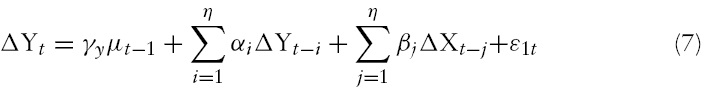
The aim of this study is to analyse housing price dynamics. Therefore, as a check for robustness, it applies the Vector Auto Regression (VAR) model. However, one area of controversy for estimating using VAR models is whether the variables included in the model should be stationary or not. Some argue that if the time series is non-stationary, then regression of one time series variable on one or more time variables can often give rise to spurious results due to the effect of a common trend. Sims (1980) and others, though, recommend against differencing even if the variables have a unit root. The main argument against differencing is that ‘it throws away’ information concerning the co-movement in the data, which in general leads to poor forecasting. However, econometricians use stationary variables for stability and robustness of results in VAR. Therefore, wherever endogenous variables are found to be non-stationary, the study considers differencing the series for its stationary values. The VAR model can be represented as follows:

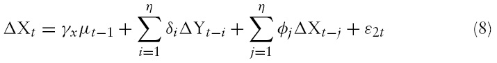
The above two equations constitute a vector auto regression model (VAR) in first differences. In equations (7) and (8), if
There are two approaches, impulse response function and variance (forecast error) decomposition, for characterising the dynamic behaviour of the VAR model. Equations (7) and (8) are rather difficult to describe in terms of
Following Sims’ (1980) seminal paper, dynamic analysis of the VAR model is routinely carried out using the ‘orthogonalized’ impulse responses, where the underlying shocks to the VAR model are orthogonalized using the Cholesky decomposition. This method assumes the system is recursive in a sense that all the determinants are influencing the housing prices simultaneously and the estimations of the impulse response function and variance decomposition are orthogonalized so that the covariance matrix of the resulting innovations is a lower triangular matrix.
[Table 1.] Results of unit root test
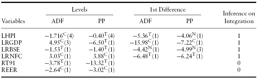
Results of unit root test
Empirical Results and Discussion
The empirical analysis reported here is based on two-stage estimation. In the first stage, cointegration analysis is used to identify the cointegrating relationship among the variables. This is important because, if two non-stationary variables are cointegrated, a VAR model in the first difference is misspecified. If the cointegration relationship is identified, the model should include residuals from the vectors (lagged one period) in the dynamic Vector Error Correction Model (VECM).
As discussed in the previous section, it is necessary to check the order of integration of the level variables for an appropriate econometrics method. Therefore, unit root tests of each variable at their levels as well as the first difference of non-stationary level variables were conducted. The results from Table 1 show that all the variables are non-stationary at their levels except RT91 (short-term 91-day Treasury bill rate) and REER. However, all the non-stationary variables are found to be stationary at their first differences, and therefore, are integrated of order one.
Cointegration ?Vector Error Correction Model
The cointegration model used here has in total six variables; four non-stationary variables, namely house price Index (LHPI); per capita real GDP (LPRGDP); real Bombay Stock Index (LRBSE); real non-food bank credit (LRNFC); and two stationary variables, namely real effective exchange rate (REER), and real State Bank of India advance rate (RSBIR). The two stationary variables have been assumed to be exogenous in the cointegration framework as they are likely to exert their influence on house prices in the long-run rather than getting influenced by other variables. Studies also show that their behaviour is quite independent of the movement of other monetary, fiscal and real influences (Nachane
The VECM involves selection of appropriate lag length. An inappropriate lag selection may give rise to problems of over-parameterization or underparameterization. The objective of estimation is to ensure that there is no serial correlation in the residuals. Likelihood Ratio (LR), Final Prediction Error (FPE), Akaike information criterion (AIC), Schwarz Information Criterion (SIC), and Hannan-Quinn criterion (HQ) are used to select optimal lag lengths. Up to three lags are tested in the present study.7 All the criteria such as LR, FPE, AIC, SC, and HQ select for the second lag. Hence, the second period is considered to be the optimal lag.
7The results are not reported here due to space constraints but can be made available upon request.
Results from Cointegration Tests
The cointegrating relationship is tested with equation (6). The relationship is estimated by the Johansen (1988) multivariate cointegration test.8 Table 2 presents the trace and maximum eigenvalue statistics for the sample period: 1996:1 to 2007:1. The test statistics and asymptotic critical values at 1% and 5% are also shown in Table 2. Both tests reject the hypothesis of no cointegration (
8In the Johansen Test, we can calculate the trace statistic, i.e. λi (0) = –T [ln (1–λ1) + ln (1–λ2) + ln (1–λ3).Where Tis the total number of observations less the lags and λi are the characteristics roots of the coefficient matrix of independent variables. Similarly, the same formula can be used in the calculation of the maximum eigenvalue statistic. See Enders (2004) for more details.
Long-run Estimates of Housing Price Equation
The long-run coefficients obtained from the cointegrating equation shows that the real income measured from real
[Table 2.] Johansen co-integration rank test
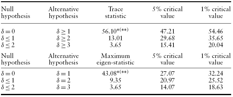
Johansen co-integration rank test

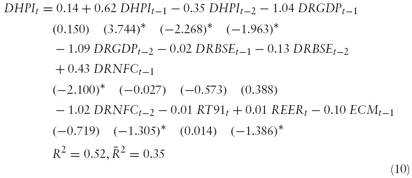
Short-run Estimates of Housing Price from VECM Model
The prefix ‘D’ in the short run equation represents delta, or changes in value of the corresponding variables used in the estimation. The coefficients of the error correction termin theVECMshowthat it is significant and it possesses the correct (negative) sign, implying that there is partial adjustment of housing prices in the short run due to its deviations from its long run equilibrium path.The adjustment is around 10% per quarter. This implies that any disequilibrium in the housing market fromits long run equilibrium takes around two and a half years to correct the disequilibrium. Looking at the short-run parameters, it suggests that both real GDP and real interest rate have a significant and negative influence on housing prices. Other variables do not play a significant role in the short run. Some of the literature argues that housing investment is long term in nature. It needs enhanced permanent income for housing investment. Even if there is a change in transitory income in the short run, the housing investment will not be stimulated unless there is an increase in the permanent income. This is the reason why a short-run rise in income does not encourage investing in/constructing housing, thereby putting downward pressure on the housing prices. It is also found that about 52% (
As a prelude to estimating in a multivariate set up of VAR, the study conducts a Granger causality test between housing prices and their determinants.9 If there exists some causality relationship among the variables in the bivariate model, then it is only meaningful to test their relationship in a multivariate framework. The results of the F-statistic suggest that all determinants including national income, Bombay Stock Exchange, and non-food bank credit Granger cause housing prices, except real interest rate (RT91) and real effective exchange rate (REER). Although no causality is observed from real interest rate and the trade-based real effective exchange rate to house prices, the reverse causality exists. A number of points also emerge from causality test results. Palanisami and Ramamoorthy (2007) have indicated that there is some evidence of inertia with the short-term interest rate, implying a decrease in the short-term interest rate causes rising housing prices in the Indian economy and vice versa. This is because the buyers enjoy a short-term floating interest rate rather than the long-term interest rate. The main effect of the interest rate on housing prices is likely to come through its effect on builders’ funding cost and buyers’ borrowing cost. The feedback effect, however, is not observed in our result. The results indicate that the real effective exchange rate Granger causes housing prices as expected, but the reverse causality effect is not observed. Although the theory suggests that depreciation in the exchange rate could push up housing prices, thismay not be the case in the short run.10 However, given these results, it makes sense to include all of these variables in a VAR framework to understand the true dynamic relationship among the variables.11
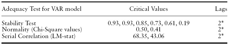
[Table 3.] Diagnostic checking criterion

Diagnostic checking criterion
To provide further insight on the relationship of housing prices and its determinants, the variance decomposition and impulse response function are computed. These two approaches give an indication of the dynamic properties of the system and allow us to gauge the relative importance of the variables beyond the sample period. Before estimating the Variance Decomposition and Impulse Response functions, one needs to ensure the model adequacy by using the required diagnostic checking procedures.
The results reported in Table 3 points out that a VAR estimated with lag two satisfies the stability test, and the normality test as well there being as no serial correlations among the residuals in the VAR model. Therefore, it leads us to take the position that our model fulfils the model adequacy tests for the statistical analysis.
9The Granger Causality test results are not produced here due to space constraint but can be made available upon request. 10According to Abelson et al. (2005), ‘In an open economy, the exchange rate could influence house prices i.e., a lowexchange rate increases the attractiveness of housing assets to foreigners.As a result, the increasing housing investment on housing will lead to rising housing prices in an economy’. 11The causality test results show that there may be a bi-directional causality relationship among two variables, but that could be due to a third common factor with which two variables are related without having true causality relations among the tested variables. Similarly, test result may show that there does not exist any causality relationship, but there could be causality between two variables once the intermediate link between the two variables is established through other variables in a multivariate framework. Therefore, it necessitates a multivariate modelling in order to discover the true direct and indirect relationship among the variables.
Variance Decomposition Results
The variance decomposition measures the percentage of variation in housing prices induced by shocks emanating from its relevant determinants.The estimates of variance decomposition are shown in Table 4 for a period of 20-quarter time horizons. The results indicate that disturbance originating from housing price itself inflicted the greatest variability to future prices. It contributes 89% variability one quarter ahead, approximately 54% five quarters ahead. The proportion of variance remains high (56%) even up to the 20th quarter. This result indicates that a current change in housing prices heavily influences people’s expectation of future price changes. Despite an average of 56% variability contributed by current price changes, there remains 44% of variability, which is explained by the other five factors.12 Total real non-food bank credit availability prevails over the other four housing price determinants in influencing house prices. This accounts for approximately 30% of the total variance contributed by five determinants (i.e. 13% of the total variance) as shown in the Table 4. This variable captures the amount of bank credit availability to households for house purchase, or for taking rented houses, as well as funds available to the builders for house construction. A relatively high proportion of housing price variance induced by credit availability confirms its importance in the dynamic behaviour of house prices.
[Table 4.] Variance decomposition of housing prices
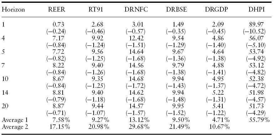
Variance decomposition of housing prices
The third largest source of housing price variance appears to be from the real BSE index, which accounts for approximately 21% of the total variance contributed by five determinants (i.e. 9% of the total house price variance). This indicates a very significant relationship between the two markets. Clearly, during the past ten years of rapid economic growth and financial reforms in India, the values of both real assets and financial assets have appreciated enormously. Thus, this implies that the stock market and housing markets are perfectly integrated. The stock market, which is highly liquid with relatively low transaction costs, is characterized by a high degree of speculative activity. It is possible that the stock market may have some influence on speculative house building and investment but this is likely to be temporary in nature.
The fourth largest source of housing price variance appears to be from the real short-term interest rate, which accounts for approximately 21% of the total variance contributed by five determinants (i.e. 9% of the total house price variance). This variable captures the cost of borrowing to households for house purchase as well as builder’s development funding cost. A relatively high proportion of housing price variance induced by interest rate confirms its importance in the dynamic behaviour of house prices. It is, therefore, not surprising that it contributes a significant proportion of house price volatility.
Apart from these three determinants, the two remaining variables account for less than 8% of total housing price variance. Real Effective Exchange Rate accounts for approximately 7% of total house price variance (that is, approximately 17% of the total variance among five determinants). However, the result indicates it is not significant.The final variable in the model, realGDP, contributes very little to housing price variance (5% of total housing price variance). The result suggests that the demand factors for the housing market have greater long-term impact than short-run impact, which is modelled in the above VECM.
12It can be emphasized that the current housing price variance (56%) is accounted for by its own house prices in India. This implies housing price is a sufficient statistic for the homebuyers; thereby, the past rise in house prices leads to the present rise in demand for housing with an expectation of a future rise in house prices, and this in turn results in a current rise in house prices. In contrast, for the house builders, the house price may not be a sufficient statistic due to the increasing costs of production, which limits the housing unit production.
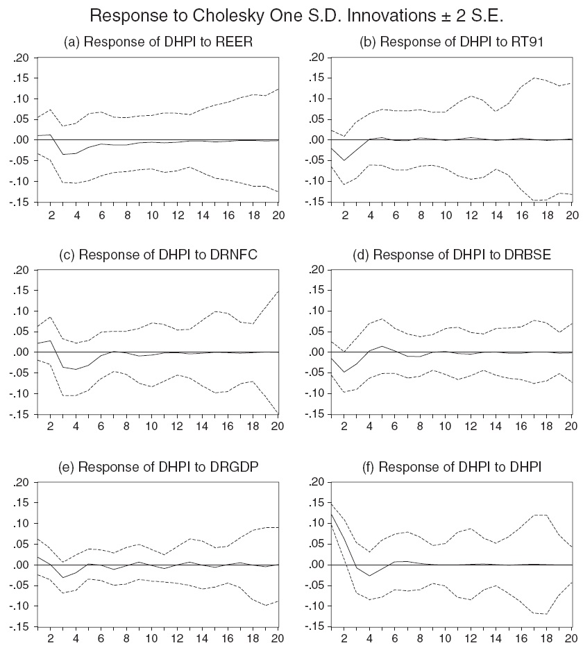
Results from the Impulse Response Function
Although the variance decomposition estimates the proportion of housing price variance accounted for by its determinants, it cannot indicate whether the impact is positive or negative, or whether it is a temporary jump or long-run persistence. Thus, impulse response analyses are carried out to indicate a system’s dynamic behaviour. They predict the responses of housing price to various shocks in its determinants. In other words, an impulse response function shows how a variable in the VAR system responds to one standard deviation shock in another variable of interest.
Figures 1(a) to (f) illustrate the estimated impulse response functions for 20-quarter time horizons. Real effective exchange rate is expected to have a negative influence on housing prices. In Figure 1(a), however, we find that real effective exchange rate results in a 0.01% increase in housing prices during the first two quarters and there is a negative response only after the third quarter. The results suggest that the appreciation of exchange rate discourages the foreign investors from taking any investment project in the economy where the exchange rate is overvalued against their currency, which subsequently leads to a reduction of housing prices in an economy.
A one-standard-deviation disturbance originating from the real interest rate in Figure 1(b) results in an approximately −0.02% decline in housing prices in the first quarter; the price adjustment, however, undergoes a reversal (−0.01 to 0.01%) between the second to fourth quarters.Given that the interest rate is often used by the monetary policy to dampen housing price inflation, a higher interest cost could both raise housing prices and also reduce demand and, consequently, causes decline in the house price. As seen in the Figure 1, the interest rate has a negative relationship mostly in the first year, implying that the chief determinant of housing prices is from the demand side in the short-run. However, the positive sign after the fourth quarter suggests that the rise in interest rate increases the builders’ cost of capital, which is subsequently reflected in higher house prices in the long run.
Real non-food bank credit in Figure 1(c) has a positive effect on housing prices as expected. It has a greater positive effect (0.03%) in the first quarter, implying that buyers’ demand for housing increases rapidly due to easy availability of credit from public and private financial institutions in India. However, in the second quarter there is a negative response in house price to a one standard deviation shock in noon food credit. This is almost similar to the previous results obtained from VECM.
A one standard deviation disturbance originating from the real stock price index in Figure 1(d) results in an approximately −0.01% change in housing prices. It initially produces a negative impact on housing prices in the first two quarters and has a large positive impact in the third quarter. The possible explanation for the positive and negative impacts could be the influence of speculative activity in the stock market spilling over to investment in the housing market. It is also feasible thatwealth created in the stock market has a positive effect on the housing market in the long run.
A one standard deviation disturbance originating from real GDP in Figure 1(e) produces an increase of 0.02% in housing prices in the first quarter; the speed of adjustment is fairly rapid and it declines after the second quarter. In response to a one-standard-deviation disturbance in its own house price in Figure 1(f), house prices increase by 0.12% in the first quarter. This appears to die out very quickly, implying that the current price change has a greater influence on people’s expectation of next quarter’s price rather than over the longer-term horizon.
This shows that result could vary depending on the methods employed for estimating the relationship, as the study finds that there are factors that could not explain in the VECM in the short run, however, found to explain with variance decomposition and impulse response function of VAR model for future years. However, there are some consistencies in the results obtained by employing different time series econometrics, making the study most interesting for further analysis in other developing and emerging economies.
Conclusion and Policy Implications
The overall aim of the paper is to investigate the long and short run determinants of housing prices and to examine the sources and the extent of housing price variability due to relevant determinants within the context of a partial macroeconomic framework. The techniques employed for analysis include Johansen’s cointegration test and VECM model and variance decomposition and impulse response techniques in the VAR.
The findings using quarterly data for the period from 1996:1 to 2007:1 indicate that there is a long-run equilibrium relationship between housing price and its determinants, including real GDP, and real non-food bank credit. The long-run coefficients obtained from the cointegrating equation show that the real GDP has a significant and positive influence on the housing price while the real BSE index does not have any influence on housing price. In addition, the real non-food credit has a significant and negative influence on housing price. The increased demand arising due to increased income is higher than the supply of houses due to increased availability of bank credit, leading to an overall rise in house prices in the economy over the long-run. The coefficients of the error correction term in the VECM show that it is significant and possesses the correct (negative) sign, implying that there is partial adjustment of housing prices in the short run to its deviations from its long-run equilibrium path. The adjustment is around 10% per quarter, implying it takes about two and a half years to fully adjust to the deviations from its long run equilibrium. Looking at the short-run parameters, it suggests that both real GDP and real interest rate have a significant and negative influence on housing prices. Other variables do not play a significant role in the short run.
In order to test the sources of variability and identify the responses of housing prices to its determinants, the study decomposed the housing price variance. The results indicate that a disturbance originating from its own housing prices induces the greatest variability in house prices: it accounts for 89% of the variability one period ahead, approximately 54% four quarters ahead and 56% six years ahead. The remaining (44%) variance is accounted for by the five determinants. The supply side factor (credit availability alone) accounts for 13% of the housing price variance and demand side factors (real GDP, real interest rate, real stock prices, and real effective exchange rate) explain another 31%.
Comparing these empirical findings with the findings in the context of developed countries, such as USA, it is interesting to note that many of the studies in the US context find that there exist cointegration between housing price and other macro economic variables, while a few studies (Gallin, 2006; Mikhed and Zemcik, 2009) find no-cointegration among the variables. To us, the explanation is that since housing has been one of the important activities for USA for many years, the return on this asset is well linked to returns on other assets in the USA. In India, however, it is only recently that one will observe the association between the macro variables and housing prices. Further, the rate of return on savings with other macro variables was absent in India until as late as the early 1990s, when financial liberalization measures were initiated along with external sector liberalization, and it is known that the interest rate variable is one of the main instruments through which the monetary transmission channel operates, besides bank credit. If the interest rates were policy controlled for several years, this implies that the effect of the monetary transmission was being neutralized. When it was liberalized along with the emergence of growth of trade in housing, then it has recently been found to have a cointegration of the housing market with the other macro economic variables. This comparison one will also find in our earlier work (see Mallick&Mahalik, 2010). However, there are reasons why few studies in the USA context report no cointegration relationship between housing prices and other macro economic variables. It is because the results depend on the different methodologies employed for different papers, the sample period studied and whether the paper is exploring the relationship in a micro context or macro context.
Further, drawing on Leamer’s (2007) work, one can expect both short run and long run impacts of the housing prices (markets) on the economic activities (construction activities) of the developed economies, but for developing economies one may observe the impact of the housing prices on economic activities only over the long run (see Mallick & Mahalik, 2010).
This can be justified by arguing that the housing sector has been widely acknowledged as a business activity in the USA and other developed economies, while this is not the case for a developing economy such as India. This is a saleable and durable hedging asset for the homebuyers, builders and financial institutions in USA. Since, in the developed markets, lots of financial institutions or entities along with the home buyers and builders are engaged in this market, any short term shock may produce a visibly large response in the market, which may not be the case for developing markets such as India. The recent global crisis is the outcome of such economic events in the USA and in developed economies, including the Middle East. In contrast, the housing sector has not been widely identified until recently as a big business activity and saleable commodity in India. It is true that the construction sector in developing economies is expected to have less influence on the business cycles, and the business cycle on the housing sector.13 It is expected to have only a long-run impact, unlike the case with the developed economies. This is greatly debated in one of our (earlier–written) forthcoming works (Mallick & Mahalik, 2010).
The results from the present study have significant policy bearings. The empirical findings show that, in the long run, real income has a positive and significant effect on housing price, while real non-food bank credit (RNFC) has an adverse impact on housing prices. This result has much policy relevance in the emerging countries’ context. It claims that for India in particular, and emerging economies in general, the adverse impact of real non-food bank credit on housing price could arise because a major proportion of credit is being utilized by investors (housing builders) for profitable investment rather than for boosting consumption demand for housing (users’ demand). In addition, this implies that the credit allocation is positively skewed towards the business investors, thereby leading to construction of huge number of houses that outweigh the existing demand for housing and eventually put downward pressure on housing prices. As a consequence, such a situation ultimately discourages the house builders not to engage themselves in housing activity in the future and, in turn, reduces demand for hiring workers for construction. The presence of speculative investors in the stock market does not lead to diversification of their gained capital to other economic activities. There are two possible reasons why the speculative investor’s investment choice is limited to the stock market in emerging markets. Unlike the developed countries, such as the US, where ‘housing’ is recognized as a business activity, in emerging markets such as India, ‘housing’ is considered as a necessary durable commodity (see Mallick & Mahalik, 2010). The recognition of housing as a necessary commodity in emerging economies does not incentivise the speculative investors for higher profits, as expected from the stock market. The other reason is that a lot of complex procedures are involved in the entry process into real estate investment in India.14 Moreover, since the supply side factor, i.e. bank credit availability, scores the second highest share of total housing price variance next to its own housing price shock, the role of bank credit cannot be underestimated in the dynamic behaviour of housing price in emerging economies such as India. This is a matter of serious concern for the government and for the policy makers of emerging economies to keep an eye on the balanced distribution of bank credit for the both the players (consumers and investors) in the housing activity and to curb the speculative nature of investment via relaxing the entry procedures, which incentivises the investment in the Indian stock market. The realization of such a proposition in India may boost the general economic activity, backed up by an improvement in the investment on residential housing activity through the channel of equal distribution of credit to the respective players in the housing market. Therefore, the findings in this study suggest that the determinants of housing prices, supply side factors in particular, should not be underestimated in the dwellings market of India and other emerging economies, as they can play important roles in the dynamic behaviour of housing prices.
13The housing sector in developing economies is also not greatly affected by business cycles. Downloaded by [Yonsei University] at 19:46 24 July 2011 14Of these two reasons, as cited in the above, the second reason seems to be the sufficient factor in the case of speculative investors in making their investment decisions. They basically prefer to invest in the stock market because it involves high windfall gains backed by a high risk in the short-run, while investing in housing requires a huge lump sum of money and it is long term in nature.