This work develops a simple framework to analyse how financial intermediaries’ balance sheet problems combined with financial guarantees make an economy more vulnerable to financial crises. A ‘double default’ problem – that is, the default of financial intermediaries on their debt repayments and of the government on its guarantees to bailout intermediaries’ losses – is modelled in this study.The possibility ofmultiple equilibria, including a crisis equilibrium where the government is not able or willing to honor its guarantees towards the domestic financial sector, arises from the interplay of all the above elements: financial intermediaries’ level of indebtedness, government implicit guarantees and high-risk creditors’ lending. This work also produces predictions concerning the vulnerability to a financial crisis: multiple equilibria are possible only in certain ranges of the fundamentals.
Third-generation models have been introduced to detect the origins of the financial crises that spread throughout emerging economies over the last decade. As it is well-known the canonical first-generation models, exemplified by Krugman (1979) and by Flood and Garber (1984), explain the crises as the product of budget deficits. Flood and Garber (1984) show that the abandonment of a currency peg will be typically enforced by a speculative attack of rationally acting market participants who try to sell the currency to avoid losses. The second-generation models, exemplified by Obstfeld (1994), explain the crises as the result of a conflict between a fixed exchange rate commitment and the desire to pursue a more expansionary monetary policy. A government decides whether it can defend a pegged exchange rate according to a trade-off between short-run macroeconomic flexibility and long-term credibility. However, the 1990s Asian meltdown suggested that the crisis might be not a problem of unsustainable budget deficits policies carried out by local governments, as in the first-generation models, nor is it a problem arising from ‘macroeconomic temptation’ as in second-generation models, but it is a problem of financial excess and then financial collapse (see Krugman, 1998, 1999; Salvatore, 1999).
Third-generation type models of financial crisis have focused on problems of panic and collapse, resulting from a shift from a good equilibrium to a bad one (Morris & Shin, 1998). As Irwin and Vines (1999, 2003) suggest this collapse is underpinned by what in the financial system made a bad equilibrium possible. In a third-generation model the source of the crisis should lie primarily in the interaction between financial intermediaries’ overborrowing and financial system fragility. For example, Krugman (1998) suggests that what went wrong in the Asian financial system contained an important element of moral hazard; he points out that the presence of guarantees provided by the government to a bank-based financial system was responsible for what has been defined Asian ‘crony capitalism’. This strand of literature argues that moral-hazard-driven lending might provide a hidden subsidy to investment, which collapses when governments are not able (or not willing) to honour the guarantees (see McKinnon & Pill, 1996; Dooley, 2000)
Irwin and Vines’ (2003) work presents a story of financial collapse by putting together Krugman’s idea of government financial guarantees with Dooley’s (2000) idea of a government-limited ability to bail out the domestic financial institutions whose liabilities were covered by such guarantees (either implicit or explicit). Aghion
The financial sector has played a central role in explaining the last decade’s crises as well as the current global crisis. The first 21st-century world-scale financial crisis has been caused by a poorly supervised bank-based financial system where the moral hazard behavior of the main market players (i.e. financial intermediaries, investment banks and also insurance companies) was in part caused by implicit financial guarantees. The global crisis had its origins in an asset-price bubble, which burst in the summer of 2007, in the US residential mortgage market where a large number of government interventions and distortions have been responsible for moral hazard behavior and excessive risk-taking by agents. In fact, many banking and financial intermediaries did not keep the mortgages on their books and repackaged them into asset-backed securities. Domestic and foreign investors considered these securities not risky because the underlying mortgagebased products benefited from either explicit or implicit guarantees from the government (Freixas & Parigi, 2010; Freixas
The paper attempts to evaluate how the evolution of the solvency of bankbased financial systems to which the government provides guarantees might explain the origin of recent financial crises. Starting from Irwin and Vines’ (2003) model, we have developed a simple framework to study how financial intermediaries’ balance sheet problems combined with bailout policies make an economy more vulnerable to financial crises. The possibility of multiple equilibria, including a ‘bad’ equilibrium where the government is not able to honour its guarantees, arises fromthe interplay of all the above elements: financial intermediaries’ balance-sheet currency mismatches, government guarantees and high-risk creditors’ lending. Our study, along the lines of the multiple equilibria models (Morris & Shin, 1998; Sachs
The building blocks of our model are the following: (i) due to the presence of government guarantees, financial intermediaries willingly expose themselves to exchange rate risk by borrowing both in domestic and foreign currency and lending in domestic currency without hedging the resulting risk; (ii) because of the currency mismatch in their balance sheets, financial intermediaries might find it optimal to renege on their debt and declare bankruptcywhen a devaluation occurs; and (iii) the government might be either unable or unwilling to fully afford the costs associated with financial guarantees and bank rescues.
The paper is organised as follows. Section 2 presents the basic model. Section 3 examines the effects that follow the introduction of government guarantees on financial intermediaries’ debt. Section 4 analyses both the short-run and longrun equilibrium solutions of the model. Section 5 presents a numerical exercise. Section 6 comments on the results and highlights the policy implications of the model. Section 7 concludes.
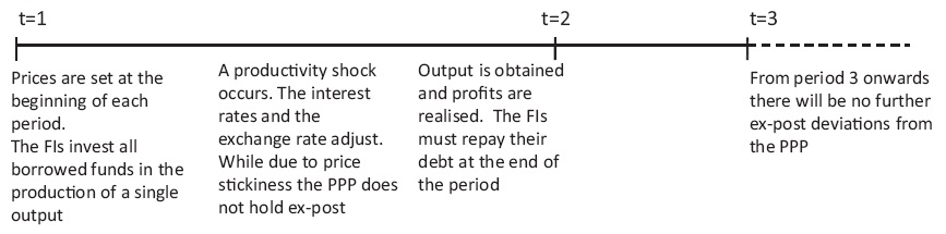
There is an infinite-horizon, small open-economywhere many Financial Intermediaries (FIs) operate; they own all the productive capital stock,which they borrow from domestic and foreign lenders and invest in the production of a single output sold in the domestic competitive market. Output price is determined at the beginning of each period t and it remains fixed for the entire period. Therefore, due to nominal price stickiness, the Purchasing Power Parity (PPP) holds only in expectations:

where

is the expected nominal exchange rate at time
Arbitrage by investors between domestic and foreign assets in a world with full capital mobility is captured by the Uncovered Interest Parity (UIP) condition:3
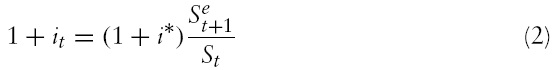
where

is the expected exchange rate in the next period,
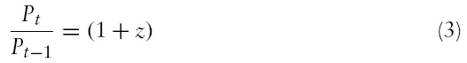
where

is the (gross) domestic inflation rate, and the parameter z denotes the constant rate of growth of money supply. Equation (3) holds for all periods without shocks, that is from period 3 onwards. In periods 1 and 2 the nominal interest rate aswell as the exchange rate,which is assumed to be perfectly flexible, adjust in response to a real shock to clear the money market while prices remain fixed until the end of the period, when they adjust.
With no shocks, the inflation rate targeting rule, equation (3), and the PPP, equation (1), imply that the nominal exchange rate evolves as follows:

Relationship (4) holds from period 3 onwards, and it follows from the assumption of absence of real shocks after period 2.
2.1 Bank Indebtedness and Capital Investments
FIs’ capital investment in each period

which pays a nominal interest rate,

which is risk-free and pays a world interest rate

where
is the real amount of debt in domestic currency and
is the real amount of debt denominated in foreign currency, with 0 ≤
Following Irwin and Vines (2003), we assume that FIs produce according to a Cobb-Douglas production function:

where
For the sake of simplicity we assume that labor is supplied inelastically at the real wage

If capital fully depreciates within one period and it is entirely financed by borrowing from domestic and foreign creditors, then FI’s capital stock at the beginning of each period is equal to:

Under equation (8), output becomes a function of the FI’s external borrowing capacity (leverage) as well as of the currency composition of its own debt:

Since we allow FI’s productivity, u, to vary in periods 1 and 2, while no further unexpected shocks occur after period 2, then productivity is constant for all
As shownin Figure 1, at the beginning of period 1 FIs invest all the capital they own in the production of a single good whose price has been preset at the beginning of the period. During periods 1 and 2 an unexpected productivity shock occurs. This causes a change in the nominal exchange rate – which is assumed to be floating – and an adjustment of the domestic interest rate. Prices are fixed and they cannot change during periods 1 and 2. At the end of each period the output is realised, FIs’ earnings are determined and debt is repaid.We allow for a negative productivity shock (i.e. a fall in the productivity) to occur only in periods 1 and 2, while in all the subsequent periods no further shocks occur and FIs’ productivity is constant and sufficiently high to allow the economy to converge to its steady state.
The FI’s end-of-period nominal net profits are equal to the difference between net output sales5 and debt repayments of principal plus interest to creditors:

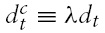
where the term

as clearly shownin equation (10).The above relationship also shows that if there is a positive productivity shock, that is if
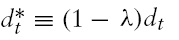
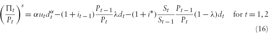
By using the relationship (10), net profits at the end of periods 1 and 2 expressed in real terms read as:6
where the real net profits,

at time
In all periods after period 2, the following equality holds:

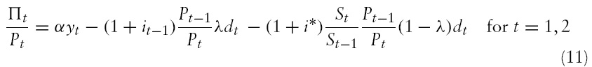
Given equation (12) and using the UIP, equation (2), and the inflation targeting rule, equation (3), real net profits from period 3 onwards read as:
where
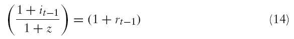
In equation (14), (1 +
Expression (13) shows that starting from time
Relationships (1) and (4) also imply that, in the absence of shocks, the domestic and foreign real interest rates will be equal:
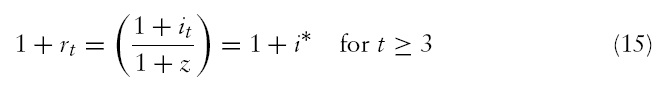
The above relationship follows from the UIP and the PPP conditions, since, in the absence of shocks the following relationships hold:

and
We have assumed that the economy converges to its long-run equilibrium after period 3; hence, we define the long-run as any period

where superscripts

for
This model also assumes that FIs have limited liability7 and no capital requirements, which implies that FIs can default without costs.Therefore, FIs can exploit all the sources of potential profit, even if the expected profits are negative. In economic models we normally think of investors as responding to expected values of the relevant variables. But if the owners of FIs do not need to put up any capital, and can simply walk away if their institutions fail, they will instead focus on the values that variables would take if it turns out that we live in what is the best of all possible worlds. This will generate a problem of overinvestment that lowers expectedwelfare, because the increased return in the favorable state will not offset the increased losses in the unfavorable state (Krugman, 1998).
By using equation (16) under the condition of zero net profits and the assumption that there is a large number of FIs that act competitively in the domestic financial market, the FI’s short-run level of indebtedness is equal to:
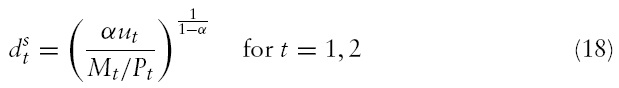
where

Relationship (18) highlights two important issues: (i) higher productivity,
From equation (17), under the zero net profit condition and the assumption made over the distribution of the productivity parameter,
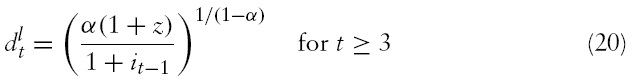
where
In the following section,we will analyse the role played by (implicit) government guarantees on FIs’ debt; such guarantees pose a serious problem of moral hazard since they affect the interest rate at which lenders are willing to lend and this, in turn, indirectly influences the FIs’ investment decisions. This story resembles the proposition that over-guaranteed and poorly regulated intermediaries can lead to excessive investment by the economy as a whole (on this point see McKinnon & Pill, 1996).
Therefore, in the following sections we will define both the long-run and the short-run equilibrium level of the nominal interest rate inclusive of the implicit government guarantees on the FIs’ debt. The government guarantees the loans (principal and interest) made to the domestic FIs and it commits itself to raise sufficient funds to repay the debt. Lenders formulate some conjecture on the possibility that the guarantee will be fulfilled by the government in the case of FIs’ insolvency, and this will affect the interest rate at which they are willing to lend. In fact, such guarantees, by artificially lowering the credit risk, influence the level of the lending rates atwhich FIs can borrowfunds. If interest rates are pushed down, a moral-hazard-driven overlending may be generated and the demand for credit goes beyond the level that is economically efficient. This will be further analysed in the following sections.
1As is commonly assumed by the existing models of open monetary macroeconomics (Obstfeld & Rogoff, 1996), the shock that occurs in periods 1 and 2 is wholly unanticipated and thus it is not taken into account by the domestic market when setting prices. 2The shock causes a deviation from the PPP in periods 1 and 2 since prices are set at the beginning of each period and remain fixed; while nominal exchange rate and domestic interest rates have to adjust to absorb the shock. 3The UIP applies with risk neutrality as it is the outcome of arbitrage fromfully diversified investors. 4This share of wages is directly determined from the Cobb-Douglas production function: yt = 5Since FIs’ produce y and pay a share of wage equal to (1 − α)y, which is determined from the assumed Cobb-Douglas production function, the resulting sales net of wage payments will be equal to αy. 6Both prices and exchange rate at time 0 have been normalized to 1. 7The assumption of FIs’ limited liability, implies that if FIs’ owners have insufficient funds to make debt repayments, they can default losing their equity investment without additional costs. 8By using equation (15), relationship (20) can be also written as a function of the exogenous and constant world interest rate:
3. Introducing Government Guarantees: Bank Over-indebtedness and the Bailout Cost
Let us introduce a financial implicit guarantee on FIs’ debt by assuming that the government may intervene to repay lenders when FIs have not enough funds to honour their debt.9 In each period the bailing out cost,

where
Using equation (21) and the PPP and UIP conditions, the long-run cost of bailout reads as:

where the term

is the long-run cost of bailout faced by the government with subscript
Similarly we can use equation (21) to define the short-run cost of bailout faced by the government:

where the term

is the short-run cost of bailout faced by the government with subscript
In each period, the government can choose not to bail out insolvent FIs when the cost of debt service,

where the overall cost of reneging on the guarantee,
The no-bailout cost might be thought of as the cost of losing credibility faced by the government when it fails to fulfil the guarantee. In fact, once the government reneges on the guarantee it is not able to credibly offer this guarantee in subsequent periods. However, as pointed above, we assume that the government is myopic and it does not care about the future so that the no-bailout cost,
In absence of shocks, the PPP and the UIP conditions allow us to rewrite equation (24) as:

where

denotes the long-run cost of reneging on the guarantee, with the subscript
The short-run cost of reneging on the guarantee is simply given by relationship (24) which holds in periods 1 and 2, that is:

where the term

is the short-run cost of reneging on the guarantee with the subscript
When the FI is insolvent and defaults, the government will intervene to fulfil the guarantee and to repay the debt only if the following condition holds in each period

Therefore, given equations (21) and (27), we can compute the threshold level of the productivity shock above which the government will fulfil the guarantee and lenders will be repaid in full. In fact, the threshold level of the productivity shock can be computed by simply comparing the cost of bailing out

above which the government will fulfil the guarantee:
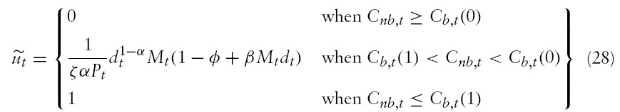
where terms
For sake of clarity, we will label relationship (28) as the Government Guarantee (GG) relationship, which describes how the trigger level of the productivity shock should vary in response to changes both in the nominal interest rate and in the FIs’ total level of debt.
3.1 Risk Premium and Interest Rates
We consider investors who have rational expectations and know that the government has a limited capacity or willingness to honour its guarantees on the FIs’ debt if things go wrong; therefore, they build up a premium into the interest rate they demand to lend to domestic FIs (Krugman, 1999; Dooley, 2000).
If lenders are rational, risk neutral and act competitively, then the domestic nominal interest rate asked on FI’s borrowing simply equals the risk-free world interest rate augmented by a risk premium that is computed as a percentage of expected default of FIs on the debt service repayments. Thus, the (gross) nominal interest rate set by creditors is a mark-up over the risk-free foreign interest rate:
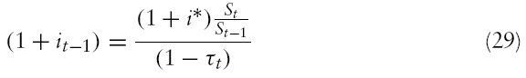
where

is the risk premium asked by lenders on FIs’ debt issued in domestic currency. Relationship (29) can be interpreted as a modified interest parity condition augmented by a risk premium. The term
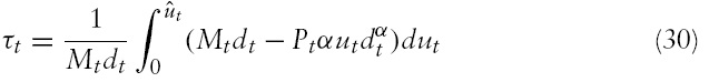
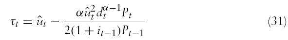
where

is the creditors’ expected threshold level of the shock above which they believe that the government will intervene to bail out insolvent FIs. In equation (30) the rate of default,

where the term

denotes some arbitrary conjecture within the range
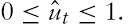
Under the UIP condition and equation (19), equation (30) can be rewritten as follows:
According to equation (31), the risk premium depends on the productivity shock, the level of FIs’ debt and the interest rate set in the previous period. As the expected trigger level rises,

the interval
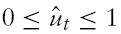
within which the government is supposed to honour its guarantees will shrink so the risk premium and the interest rate on FI’s borrowing will rise.
By plugging equation (31) into equation (29) and solving for the domestic interest rate, we can rewrite the risk premium adjusted interest parity condition as follows:
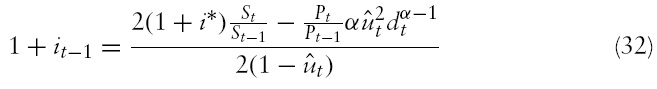
Relationship (32) shows that the domestic nominal interest rate set by the creditors is a function of the threshold level of the productivity shock,

above which creditors expect that the government will intervene to bailout the FIs,while the trigger value,

defined in equation (28), is the actual productivity shock above which the government will honour the guarantee. In order to find a closed form solution to the model wemust solve the system formed by equations (28) and (32) by imposing the condition that in equilibrium

We denote the above relationship as the Modified Interest Parity (MIP) condition since it resembles the (actual) UIP augmented by a risk premium that accounts for the FIs’ default on debt repayments. The percentage of default depends both on the expected net revenues of the FIs and on the probability that the government will not renege on its guarantees. In fact, as shown in equation (32) the threshold level of the productivity shock,

above which creditors expect that the government will bailout the distressed FIs, influences the interest rate set by lenders on FIs’ borrowing. Note that as

rises, the range of the productivity parameter values where the promises of a bailout will be honoured shrinks, this is captured by the denominator of equation (32). This implies that the probability of FIs’ default increases and thus the nominal interest rate on lending will be higher since the risk premium increases. But this effect is dampened because, as productivity raises, profits are positive and the expected percentage of FI’s default decreases as captured by the quadratic term in the numerator of equations (31) and (32).This ‘double default’ problem, that is the FI’s default on debt repayments and the possibility that government might renege on its guarantees of bailing out the distressed FI, is crucial in our analysis. In fact, rational investors do know government’s limited capacity or willingness to pay up on its guarantees in case of FI’s default and they build up a risk premium into the price at which they are willing to lend. This implies that lenders will set an interest rate over and above the world interest rate, thus reducing the long-run equilibrium level of FIs’ capital stock. The endogeneity of the risk premium poses, in our model, a multiple equilibrium problem, as shown in sections 4 and 5. In fact, the risk premium enters nonlinearly into the model, giving rise to multiple equilibria. A financial crisis might occur when a real shock shifts the economy to a bad (i.e. a ‘crisis’) equilibrium.
The model is now fully laid out and we can determine the short-run and longrun equilibrium levels of the nominal interest rate and of the trigger value of the productivity shock for government intervention establishing whether and when multiple equilibria exist.
99The assumption is that government guarantees cover both principal and interest repayments. 10This can be thought as one way of financing lending of last resort operations. There are several ways of carrying out lending of last resort facilities and, for the purpose of the model, the easiest alternative is a lump-sum tax, including the issue of new public debt to distribute this tax over a longer period. The injection of domestic currency by the Central Bank is not considered in this analysis since such an injection of liquidity by driving up prices might have feedback effects on the exchange rate.
4. Short-run and Long-run Equilibrium
In order to compute the short-run level of the (gross) nominal interest rate and the trigger value of the productivity shock for government intervention,we restate equations (28) and (32) using the relationship for the FIs’ level of debt as defined in equation (18).
Substituting the short-run level of FI’s borrowing, equation (18), into equation (23) and using condition (27), the short-run trigger value of the productivity shock,

reads as:
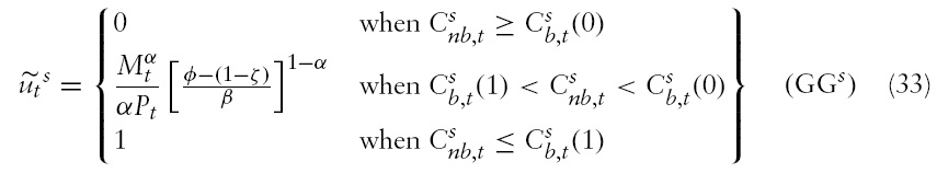
where the superscript s indicates the short-term that refers to periods 1 and 2. Relationship (33) is defined as the short-termGovernment Guarantee curve,GG
Substituting the short-run level of FI’s borrowing, equation (18), into the risk premium adjusted interest parity condition (32), we get the short-term (gross) domestic nominal interest rate:11
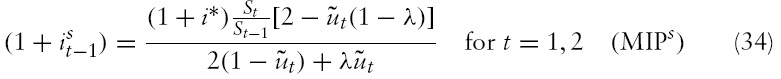
Relationship (34) is a continuous function in the domain
when
The first and second derivatives of theGG

and another at

The fact that in the short-run the trigger level of the productivity is not decreasing with respect to the domestic nominal interest rate, can be explained by the existence of arbitrage opportunities for the FIs when they issue both domestic and foreign currency denominated debt. In fact, as the domestic interest rates rise, the FIs can issue higher levels of (less costly) foreign currency denominated debt.While, the first and second derivatives of the MIP
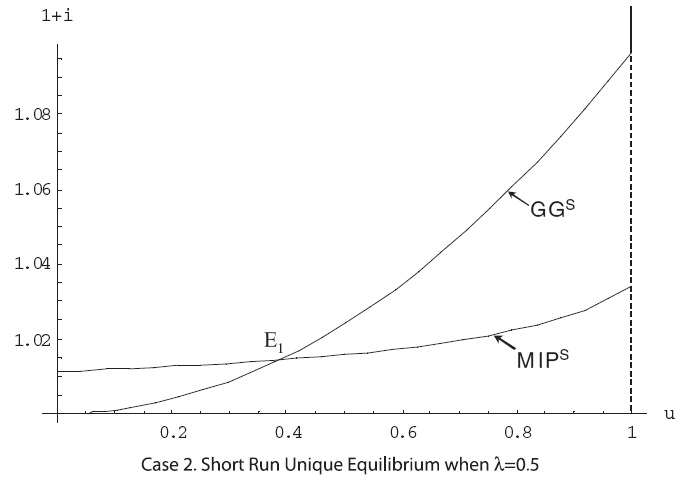
In the following section we will plot both the GG
space. The first and second derivatives of the GG
diagram are both positive sloping and convex curves (see Figures 2–4).
To compute the long-run values of the interest rate and of the trigger level of the productivity shock, we use equation (20) to substitute the long-run level of debt,

reads as:
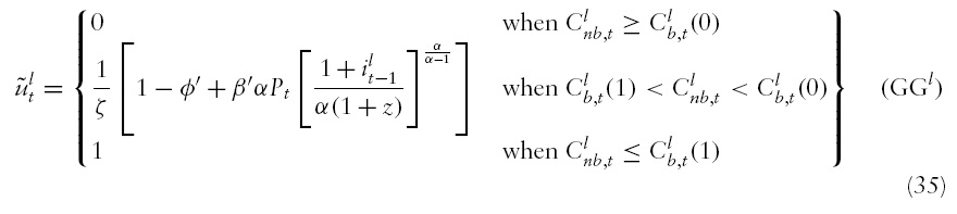
where the superscript
The relationship for the long-run gross nominal interest rate is:
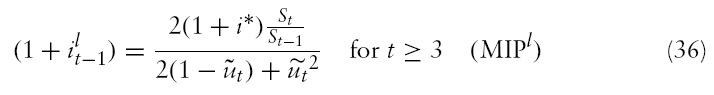
In equations (35) and (36) the term

denotes the long-run level of the productivity shock

while the term
TheGG
diagram, we express the GG

(seeAppendix B). As shownin the following section, a unique interior equilibrium exists; a condition for this to happen is that the MIP
is increasing in the trigger level of the productivity shock for government intervention,

whilst

is decreasing in
This is sufficient to ensure a unique point of intersection.
Proposition 1

11As recalled in the previous section both prices and the nominal exchange rate at time 0 have been set equal to 1.
5. Plotting the ‘Government Guarantee’ and the ‘Modified Interest Parity’ Curves
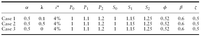
In this sectionwe provide additional insight into the analytical results by performing a numerical exercise of the basic model. Starting with the short-run period and setting the parameters with the values reported in Table 1, we graphically report both the MIP
[Table 1.] Parameter values for the short-run MIP and GG functions plotted in Figures 2?4

Parameter values for the short-run MIP and GG functions plotted in Figures 2?4
The short-term equilibrium solutions for the interest rates and the trigger level of the productivity shock are simply determined by the intersection of the GG

tends to 1, thus confirming creditors’ expectations.Therefore, in the configuration with multiple equilibria the switch from the higher interest rate interior solution equilibrium at point
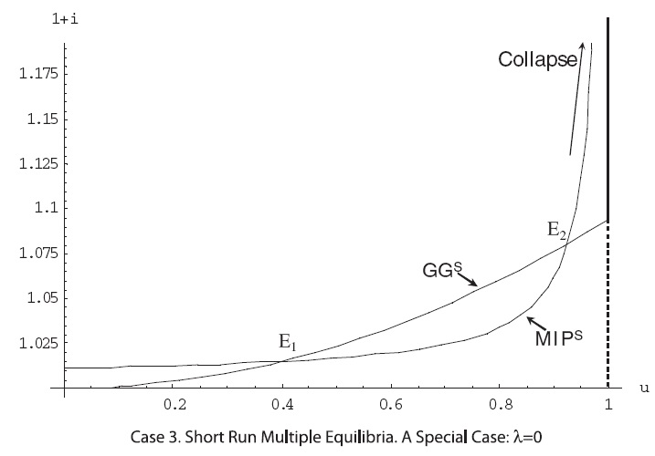
Figure 3 shows that with a cost of reneging on the guarantee,

But as depicted in Figure 3, the MIP
Another case ofmultiple equilibria is depicted in Figure 4,where theGG

u increases, and tends to infinity as

approaches 1 (see Appendix C). Figure 4 shows thatmultiple equilibriamay exist, analogously to the graphical representation of Case 1 in Figure 2. As before, with a cost of reneging on the guarantee,

approaches 1. If the economy flips away from point
Like in Morris and Shin’s (1998) analysis, there is some tripartite classification of the fundamentals that gives rise either to multiple equilibria or to a unique equilibrium scenario. In fact, by setting
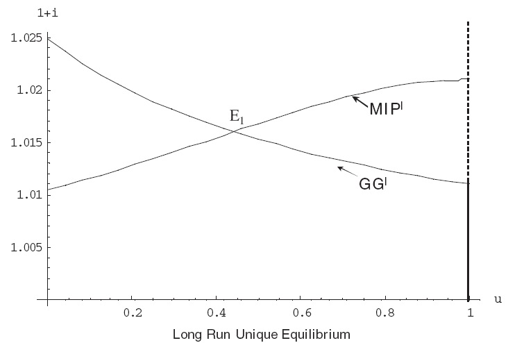
Finally, the long-run GG
Figure 5 shows that the function GG

where the interest rate is low13 and the financial guarantee is fully credible. Therefore, we conclude that in the longrun a unique equilibrium does exist and it can be either a boundary solution with a fully credible guarantee of bailout, or an interior solution with a partially credible guarantee of bailout. But as long as we assume that after period 2 no further productivity shock occurs, the long-run equilibrium will be a low-interest rate interior solution equilibrium with a trigger level of government intervention different from zero. In fact, after period 2, both the PPP and the UIP conditions hold, implying that no arbitrage opportunities exist for the FIs, so that they are completely indifferent to borrowing in foreign and/or in domestic currency and the parameter
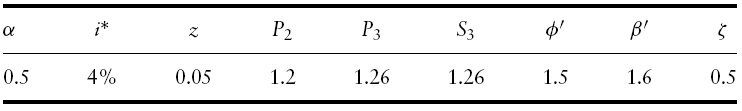
[Table 2.] Parameter values for the long-run MIP and GG functions plotted in Figure 5

Parameter values for the long-run MIP and GG functions plotted in Figure 5
This lowers the cost of guarantees, so that a government can fulfil them in a larger proportion of circumstances and the ‘good’ equilibrium, with no collapse, will be the most likely outcome as illustrated in Figure 5.
12As the threshold level of the productivity shock, above which creditors expect that the government will intervene to bailout the FIs, increases then the risk premium, τ , given by relationship (31) rises and the implied nominal interest rate on lending, equation (29), will be higher. 13At this long-run boundary solution equilibrium, the domestic interest rate is equal to (1 + i*)
6. Model Results and Policy Implications
In our analysis the mechanism that generates a financial crisis relies entirely upon the interplay of private sector behavior (both financial intermediaries and investors) and the public sector behavior (governments). Implicit government guarantees on FIs’ debt in the presence of an unregulated financial system in which financial intermediaries can default on loans at no cost might induce the FIs to increase their debt exposure, exploiting the low level of the interest rate. And investors are more willing to lend to the FIs since they know about the existence of implicit government guarantees on FIs’ borrowing. The presence of guarantees means that as bank leverage and default risk increase, the true cost to the provider of the guarantee (here the government) rises, but the cost to the bank does not. Hence, banks have the option to increase leverage to very high levels without incurring higher costs of default.
But agents know the limited capacity or willingness of the government to fulfil the guarantees and thus they lend to the FIs at a mark-up over the risk free foreign interest rate. This is captured by a risk premium adjusted interest parity condition introduced in the model. Therefore, if investors believe there is a range of productivity shocks that will force the government to renege they will ask for a higher risk premium, raising the interest rate on lending over and above the risk-free world interest rate. And if lenders raise the interest rate sufficiently it might be that the government has no choice but to renege, thus validating the (higher) risk premium so a crisis occurs. Similar to other studies that follow a multiple equilibria approach, in our model a self-fulfilling crisis might occur given the endogeneity of the risk premium on loans. But, with credible guarantees, interest rates are kept low and the government is more likely to afford and to pay up on its obligations in case of default. Like fundamentals-based models, our analysis also predicts that balance sheet currency mismatches of highly leveraged financial institutions are crucial in explaining the outbreak of a crisis. A large enough depreciation of the current exchange rate leads to an increase in the foreign currency debt repayment obligations, and consequently to a fall in profits that might induce FIs to default when the share of the foreign over domestic debt is high enough. Therefore, either changes in expectations on future exchange rate or an unexpected real shock (a productivity shock in our model) that reduce FI’s networthmay result in less investment and less output in the next periods and this brings a domestic currency depreciation, further amplifying the real shock. This basic story is very similar to the credit-based models of currency and financial crisis (see Aghion
In addition, the public sector might exacerbate the problems of the private sector; in fact, the presence of implicit guarantees on FIs’ debt repayment and the possibility that a government might not fulfil these obligations leaving the FIs to default are crucial in moving the economy to a crisis equilibrium. The investors are aware that the government promises are only partially credible and this credibility relies heavily on their conjecture about the threshold level of the productivity shock, above which the government is supposed to intervene and bail out the distressed FIs. Therefore, agents’ expectations might push up the risk premium and the interest rates if they believe that the likelihood that such (public) obligations will not be honoured is low. This lack of public sector credibility is another important feature of the model.
Previous financial crises have seen the wide use of government blanket guarantees to the financial system. While the guarantees brought stability, they limited the subsequent options for dealing with financial distress. In fact, these guarantees create complacency, delay the restructuring, while increasing the (fiscal) costs (Bank for International Settlements, 2009). The lessons from the Asian crisis suggest that blanket guarantees may have adverse consequences for financial system stability. A reason for this is that government guarantees help to stabilise sizable systemic financial crises although they do not instill market discipline. In fact, governments cannot allow banks to fail for fear that the collapse of one will cause a systemic crisis. Our work highlights that regulators should remind themselves that guarantees are a double-edged sword. On one hand, they are necessary and helpful tools in the event of a systemic crisis both for political reasons and for efficiency considerations. On the other, they might impinge on the process of reforming the financial markets in order to prevent a recurrence of global financial crises. In fact, recent theoretical literature points out that governments limit their policy options by implementing blanket guarantees that extend forbearance and increase moral hazard – a greater willingness of creditors and debtors to take the risks of such crises (Irwin & Vines, 2003). Paradoxically, government guarantees make banks and the economy less stable, not more stable. This is consistent with some empirical evidence provided by Demirgüç-Kunt and Detragia (2002) who highlight that government guarantees are detrimental to bank stability.
The financial sector has a central role in explaining the more recent crises. The end-of-20th-century financial crises as well as the current global financial crisis have originated in poorly supervised bank-based financial systems, where the moral hazard behavior of the main market players (i.e. financial intermediaries, investment banks and also insurance companies) was in part fuelled by implicit financial guarantees.
A ‘double default’ problem, that is the default of FIs on their debt repayments and of government on its guarantees to bailout FIs’ losses, is modelled in thiswork by analysing how it affects the interest rates set by investors. We show how (i) financial intermediaries’ level and composition of debt, (ii) guarantees from the public sector and (iii) moral-hazard-driven creditors’ lending could make an economy more vulnerable to financial crises. In fact, the presence of guarantees means that as banks’ leverage and default risk increase, the true cost to the provider of the guarantees (here the government) rises, but the cost to the intermediaries does not. Hence, banks have a free option to increase leverage to very high levels. In addition, this analysis takes into account the increasing cost of financial intermediaries’ debt repayment, when a currency depreciation occurs by modelling a balance sheet currency-mismatch problem. The presence of guarantees on FIs’ debt repayment and the possibility that a government might not be able or willing to fulfil these obligations, leaving the FIs to default, are then crucial in moving the economy to a ‘crisis’ equilibrium.