The wave of globalisation gave rise to a number of regional economic arrangements, particularly after the demise of the Cold War. The second half of the twentieth century witnessed a major growth of regional economic cooperation and trading arrangements. The notion of economic regionalism rapidly became vital in international trade aswell as regional diplomacy (Schiff&Winters, 1998). Although the degree of integration and cooperation varied between groups, economic regionalism ranged from a simple initiative of economic cooperation to an economic union. The growing number of regional arrangements indicated a rapid regionalisation of the global economy. Notwithstanding, the debate over regionalism versusmultilateralism continued (Panagariya, 1999a; Baldwin, 2006).
The body of theoretical and empirical literature suggests mixed results of regionalism in terms of trade flows and welfare effects (Panagariya, 2000; Limão, 2007; Adam & Moutos, 2008). Now, the fundamental questions pertaining to regional groups are as follows. First, is there any significant potential of expanding intra-group trade, which can serve as an economic incentive behind a bloc? Second, does a preferential liberalisation within the regional arrangement result in non-trivial mutual gains? This paper intends to respond to these queries in the context of an emerging regional bloc, Bay of Bengal Initiative for Multi-Sectoral Technical and Economic Cooperation (BIMSTEC), which combines seven geographically contiguous South and Southeast Asian countries: Bangladesh, Bhutan, India, Myanmar, Nepal, Sri Lanka and Thailand. The bloc was formed in 1997, and it is currently heading towards a Free Trade Area (FTA). The Framework Agreement for BIMSTEC FTA was signed in the sixth Ministerial Meeting in 2004 and was finalised in the 18th Trade Negotiating Committee (TNC) Meeting in Thailand on 4 June 2009, in which the Rules of Origin (ROOs) and Operational Certification Procedures for the ROOs were agreed. The Agreement on Cooperation and Mutual Assistance in Customs Matters for the FTA was also finalised at the Meeting. The negotiation of agreements on services and investment is in progress. However, negative lists have not yet been exchanged thus far. The FTA is expected to commence from 1 July 2012.
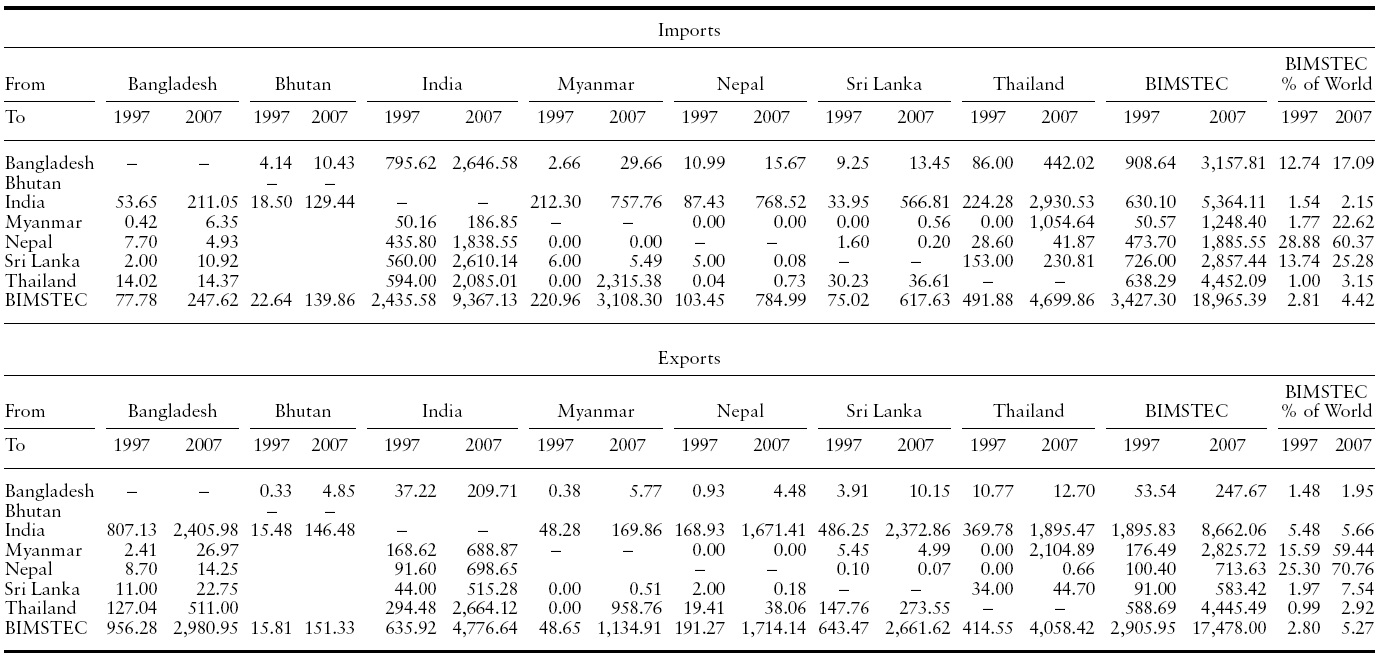
The intra-BIMSTEC trade is currently low compared with the bloc’s trade with the world. However, the magnitude of trade of member countries as well as their share in world trade increased substantially after establishing the bloc (see Table 1), which indicates increasing relative importance of this bloc even before undertaking any liberalisation scheme.1 However, trade potential remains untapped due to tariff and non-tariff barriers, and to the absence of agreements on liberalisation of services and investment. The economies are also incurring significant losses in terms of their volume and share in the economy due to the existing tariff structure. Kee
Empirical studies of the trade potential and the effects of a preferential liberalisation in the bloc are limited. Only four studies have been conducted thus far after the formation of BIMSTEC. Warr (2005) calculates intensity, bias and complementarity indices to examine Bangladesh’s potential gains for exportables. He concludes that BIMSTEC countries are not ‘natural trading partners’ and net benefits fromtrade-creating effectswould be small for Bangladesh.2 Bhattacharya and Bhattacharyay (2007) assess the trade potential of BIMSTEC countries that contextualise a BIMSTEC–Japan FTA. They find significant trade gains of BIMSTEC countries aswell as of Japan in different scenarios using a gravity model, in which the most preferable is a free trade regime. However, their approach suffers from a major drawback. The trade effect is not only related to tariff elasticity, but rather a reduction of tariff rate creates an enhancing impact on imports through three magnitudes: price elasticity of both imports and exports as well as the elasticity of substitution.
[Table 1.] Intra-BIMSTEC trade flows (US$ million)

Intra-BIMSTEC trade flows (US$ million)
Strutt (2008) makes projections for 2001–2020 that demonstrate that BIMSTEC’s total exports and imports, as proportions of those of the world, as well as intra-bloc trade, would increase. Using version 6 of the GTAP database,3 the study creates scenarios for normal track products following the Framework Agreement of BIMSTEC FTA. The study reveals that in the scenario of welfare decomposition for 2020, Bangladesh loseswelfare of US$ 267 million,whereas the welfare gains for India, Sri Lanka and Thailand are US$1.31 billion, 276 million, and 1.30 billion respectively. As a whole, BIMSTEC’s total gain is estimated to be US$2.74 billion. The terms of trade effect is included in the total welfare in CGE (Computable General Equilibrium) modelling, whereas it is not included in trade effect in partial equilibrium modelling. The main drawback of this study is that it does not explain the negative allocative efficiency effect, although the theory suggests that the tariff removal leads to allocative efficiency gain. Moreover, the Agreement in Goods was finalised in June 2009. This implies that the timing of the liberalisation tracks as indicated in the Framework Agreement cannot be attained, and the results bear a modest significance. Conversely, keeping in mind the dynamics of the global economy including the current economic crises, such a long-term projection based on an uncertain track cannot be very reliable.
Gilbert (2008) also examines the aggregate welfare effect of BIMSTEC countries using GTAP (Global Trade Analysis Project) Database 6 to assess the impact of the proposed FTA on poverty. The study reveals almost the same results of Strutt (2008). This study also suffers from the shortcomings of Strutt. Moreover, this study reports only the allocative efficiency and terms of trade effects in the welfare decomposition, but the equivalent variation is composed of investmentsavings effect along with these two effects, which is missing. It reveals net welfare loss for Bangladesh and Sri Lanka from the BIMSTEC FTA. However, their studies are based on an old database, inappropriate timing of the liberalisation phases and lack of explanation on allocative efficiency effects due to BIMSTEC FTA that contradicts the theory.
The paucity of substantial empirical investigation on the intra-BIMSTEC trade potential and possible effects of BIMSTEC trade liberalisation scheme means that further study is important to examine these aspects thoroughly. It is imperative not only to comprehend the underlying economic incentives for the liberalisation, but also to help devise appropriate policy instruments in order to facilitate the future integration scheme. Given this backdrop, the present paper is intended to re-examine the results of the previous studies with new data, to analyse the possible outcome based on estimated elasticity values of export supply, and to suggest policy recommendations based on the insights of the findings. In so doing, the possible effects of economic integration for a full tariff elimination scenario of BIMSTEC FTA are worked out in partial equilibrium and CGE models. It adopts the Software on Market Analysis and Restrictions on Trade (SMART), a partial equilibrium simulation tool, which is based on World Integrated Trade Solution (WITS).4 Complementarily, it also adopts the GTAP model to capture the welfare and trade effects based on the new database. However, the scenario of full liberalisation is not exactly the same as the liberalisation episodes in BIMSTEC FTA, but it presents a sketch of the highest possible magnitudes of its effects.
The main contribution of the paper is threefold. First, it adopts two complementary approaches, SMART and GTAP models, in calculating the
1Kabir and Salim (2010) reveal that export enhancement effect of BIMSTEC is 28.53%. 2Summers (1991) argues that when the members of trading arrangements are natural trading partners, i.e. they trade substantially with each other and are geographically proximate; the risk of trade diversion becomes minimal. However, Bhagwati and Panagariya (1996) systemically demonstrate that the hypothesis of natural trading partners does not have any analytical basis. 3It comprises 87 regions and 57 sectors and specifically Bangladesh, India, Sri Lanka and Thailand of theBIMSTECmembers separately andMyanmar, Bhutan and Nepal in the other regional groups. 4SMART adopts the partial equilibrium model described in Laird and Yeats (1986, 1990). In the literature, the model is frequently referred to be ‘SMART model’.
The SMART simulation model is used in WITS, developed jointly by the United Nations Conference onTrade and Development (UNCTAD) and theWorld Bank. It is an interactive web-based system that uses UNCTAD’s Trade Analysis and Information System (TRAINS) database, which includes a wide range of trade data classified on product categories and sub-categories. Data on tariffs are available at the most detailed commodity level of national tariffs,
The WITS uses values of import demand elasticity on disaggregated commodity groups available in Stern
The following export supply function is adopted to estimate the aggregate price elasticity:

where
For estimating equation (1), data are gathered over the period 1980–2006. The time series of annual average official exchange rate (local currency for one US dollar),
The GTAP model is described in Hertel (1997). In the model, all markets are assumed to be perfectly competitive. The regional government can drive wedges between prices of the producers and consumers by imposing taxes and subsidies on commodities and factors. Buyers differentiate between home-grown and imported goods, and also different sources of imports by region of origin. Investment in each region comes from a global pool of savings wherein each region contributes a fixed proportion of its income. Investment allocation is made according to the existing relative rates of return (Siriwardana & Yang, 2008).
In the basic analysis of welfare changes, the standard GTAP model features a representative household of a region (country). Its behaviour is governed by an aggregate utility function, which is specified over private household consumption, public expenditure and savings per capita. The GTAP simulations compute the welfare change as equivalent variation (
5A similar model has been adopted by Milner et al. (2005) who use the estimated values of demand elasticity by Stern et al. (1976) and rely on Armington’s elasticity of substitution. 6The procedure of calculating XRER is as follows. At the first stage, the bilateral exchange between individual countries (i) and their major export countries (j) (listed in Appendix Table 2), ERij, is calculated. This is used to calculate real bilateral exchange rate in the following way: where, Dj and Di are GDP deflators of destination and local countries respectively. Then an RER index has been calculated, taking 1995 as base year as follows: Finally, the weighted average of RERIij is used to construct an export-weighted XRER for home countries according to their export shares such that
3. Empirical Analysis and Findings
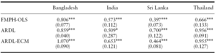
The long-term estimates of the export supply elasticity can be obtained by using the Fully Modified Phillips-Hansen (FMPH) OLS and the Autoregressive Distributed Lag (ARDL) model, while an error correction version of the ARDL can provide the short-term estimates. Among the previous studies, Athukorala and Riedel (1994), Sinha (2001), and Rao and Singh (2007) apply the FMPH-OLS in trade modelling. The ARDL has been adopted by Bahmani-Oskooee and Kara (2005) and Chen (2008).7
For the unit root test, Augmented Dickey–Fuller and Phillips–Perron tests have been performed. The results reveal that the variables used in this model are
To carry out cointegration analysis, the selection of the maximum order of vector autoregression (VAR) is important, because the result is sensitive to the choice of the order. Taking the order arbitrarily might thus provide the wrong conclusion about the number of the cointegrating vectors. Pesaran and Pesaran (1997, pp. 292–293) notice that there is a risk of over-parameterisation in taking higher order of VAR from various competing criteria, such as Schwarz Bayesian criterion (SBC) and Akaike information criterion (AIC), for a short time series. In the present case, the order of VAR is 1 based on SBC. However, only one cointegrating relationship has been found among the variables for all countries except India. For India, however, there is one cointegrating vector for restricted intercept and no trend. We rely on the maximum eigenvalue test for Bangladesh and Sri Lanka since the results vary between maximum eigenvalue and trace tests, as Johansen and Juselius (1990) suggest that the earlier test performs better.10
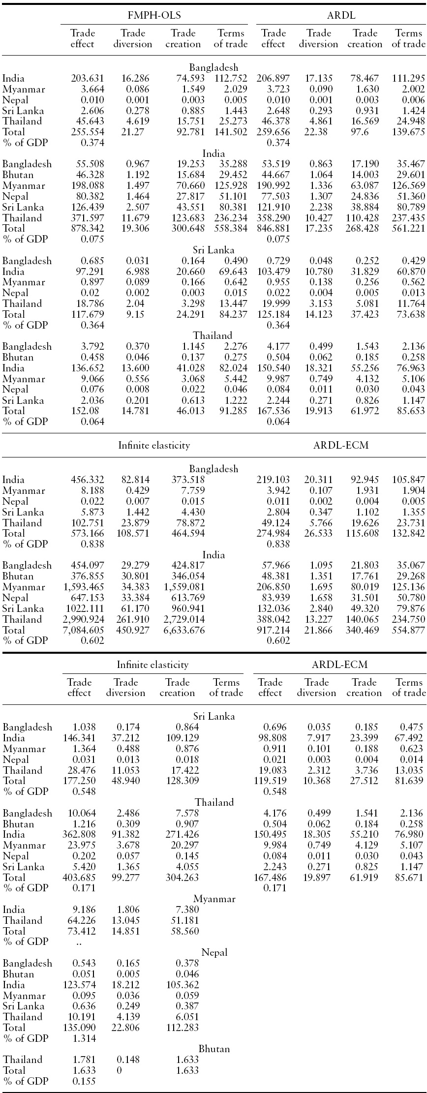
The price elasticity of export supply has been found to be positive and significant at1%level for all countries except for India in theAutoregressive Distributed Lag (ARDL) long-term estimate (Table 2).11
Various estimates of the export supply elasticity for BIMSTEC countries have been used vis-à-vis an infinite elasticity for simulation of trade effects of forming an FTA within the bloc. The values of import demand elasticity are taken from Kee
The trade effect of BIMSTEC FTA is reported in Table 3. The results indicate that it does not vary substantially for simulations based on estimated export elasticities, but differs notably between that of the estimated and infinite elasticity values except for Sri Lanka.The trade effect is the highest for India, and the lowest for Sri Lanka. The results, however, vary according to the size of the economies, trade volume, import demand elasticity and tariff regime. The import demand elasticity is the highest for India in Kee
[Table 2.] Export supply elasticity of BIMSTEC countries
Export supply elasticity of BIMSTEC countries
The FTA would result in the highest imports of Bangladesh from India among the BIMSTEC countries, followed by Thailand, but Bangladesh’s export to these countries would be much lower than imports. This implies that an FTA would further increase Bangladesh’s trade deficit with these countries. India’s trade effect would be the highest with Thailand followed byMyanmar, Sri Lanka and Nepal respectively. However, India’s exports to Sri Lanka and Thailand would be lower than its imports fromthese countries. Sri Lanka’s trade effectwould be the highest with India, followed byThailand.The FTAwould increase imports fromThailand at an amount much higher than exports. Thailand’s trade effect would be the highest with India; it would be more than 90% of its total trade effect based on short- and long-term elasticity estimates.
The results indicate that the majority of trade effects come from the terms of trade gain for all the countries in all export elasticity values. This implies that a preferential tariff elimination results in lower price of goods produced in BIMSTEC than the similar goods produced outside the bloc.12 This increases exports of BIMSTEC members and improves their terms of trade.
The simulation results, however, reject Panagariya (1999b), who argues that by eliminating tariffs preferentially from the SAARC (South Asian Association for Regional Cooperation) countries and keeping the tariff on the ROW as it was before, Bangladesh would become net trade diverting.13 Further, Panagariya (2003, p. 1283) notes,
[Table 3.] Decomposition of trade effect (US$ million) for different export price elasticity

Decomposition of trade effect (US$ million) for different export price elasticity
Here, trade creation effect is found to be much larger than diversion for all the member countries, which supports previous studies such as Calfat and Flôres (2006) and Zhao (2008). Our results confirm the international competitiveness of export items of source countries other thanBIMSTEC, and indicate that the bloc’s imports would not experience any major distortion due to discriminatory tariff liberalisation. The results further demonstrate that India’s trade creation effect is the highest among the members. The country’s trade creation effect is around 15 times higher than diversion, which is 3 to 4%for the other countries. This clearly indicates that BIMSTEC FTA leads the Indian consumers to a significantly higher level of consumption.
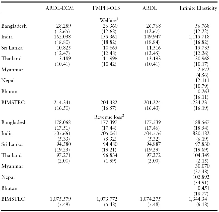
[Table 4.] Welfare and revenue loss effects (US$ million)

Welfare and revenue loss effects (US$ million)
The assumption of infinite elasticity makes significant changes in India’s net trade effect. India’s imports from the other members increase substantially. Whereas in the other elasticity scenarios Myanmar’s export effect is the second largest, in this scenario Nepal’s export effect substantially surpasses Myanmar’s export effect by taking the second position. For the other countries, the trade effect remains almost the same except for the rise in the magnitude of export effect of the top partner. In this case, the trade creation effect is much higher than diversion. This indicates that the elimination of tariff for BIMSTEC members reduces the relative price of the goods produced in the group compared with similar products in the ROW. This leads to a steeper relative price of the products given the initial level of consumption, resulting in a new equilibrium level of trade wherein intra-BIMSTEC imports increase while imports from the ROWsymmetrically decrease. Lowering the tariff for BIMSTEC decreases the domestic price of its items imported to a member country, thereby creating a revenue effect for which a country’s consumers arrive at a higher level of consumption associated with increased imports from BIMSTEC at the initial level of expenditure. This is the trade creation effect in the present analysis.
The magnitude of the welfare effect also does not vary significantly among the scenarios created based on different elasticity estimates, although it does so in the infinite-elasticity based simulation for countries, except for Sri Lanka (Table 4). It is more than double for Bangladesh and Thailand and, on average, three times for BIMSTEC in the later scenario. On the whole, India’s trade and welfare effects are both much higher than other member countries. Despite being the second largest economy in the group and trading in a wide range of products, Thailand’s meagre welfare gain is due to its lower average applied tariff rate on highly traded items.
Amongst the countries of the bloc, India’s increase in imports, revenue loss and welfare gain is the highest. This is because of its increase in the amount of imports from the bloc and the associated changes in preferential tariff elimination on a diverse category of products. In terms of the ratio of revenue loss in total revenue, Sri Lanka’s relative loss is the highest in the region followed by Bangladesh; both are smaller economies. Although India’s absolute loss is the highest, it is hovering at 6% of the total revenue, which is meagre. But the smaller countries in the group have to sacrifice around one-fifth of the total tariff revenue for the FTA, which is significant. Nepal’s trade effect is nearly double Myanmar’s effect. Nepal’s trade gain comes from all the other BIMSTEC members due to its trade relations with them, although most of the trade creation and diversion effects originate from India – the country’s overwhelmingly major trade partner. Most ofMyanmar’s trade effect stems fromThailand, the country’s major trade partner in the group.
Myanmar’s possible welfare effect is much lower than that of Nepal, both in magnitude and its share in net trade effect, although Myanmar is bigger than the later in terms of the size of the economy and its total world trade. This is because the country is less integrated with the South Asian economies. It also loses less revenue than Nepal, which is owing to its less restrictive trade regime. While Nepal’s revenue loss is more than half of the existing total revenue, Myanmar’s loss is slightly higher than a quarter. Although meagre, Bhutan’s welfare effect is proportionately higher in the trade effect than that of Myanmar and Nepal, although its relative revenue effect is similar to that of Bangladesh and Sri Lanka.
According to Kee
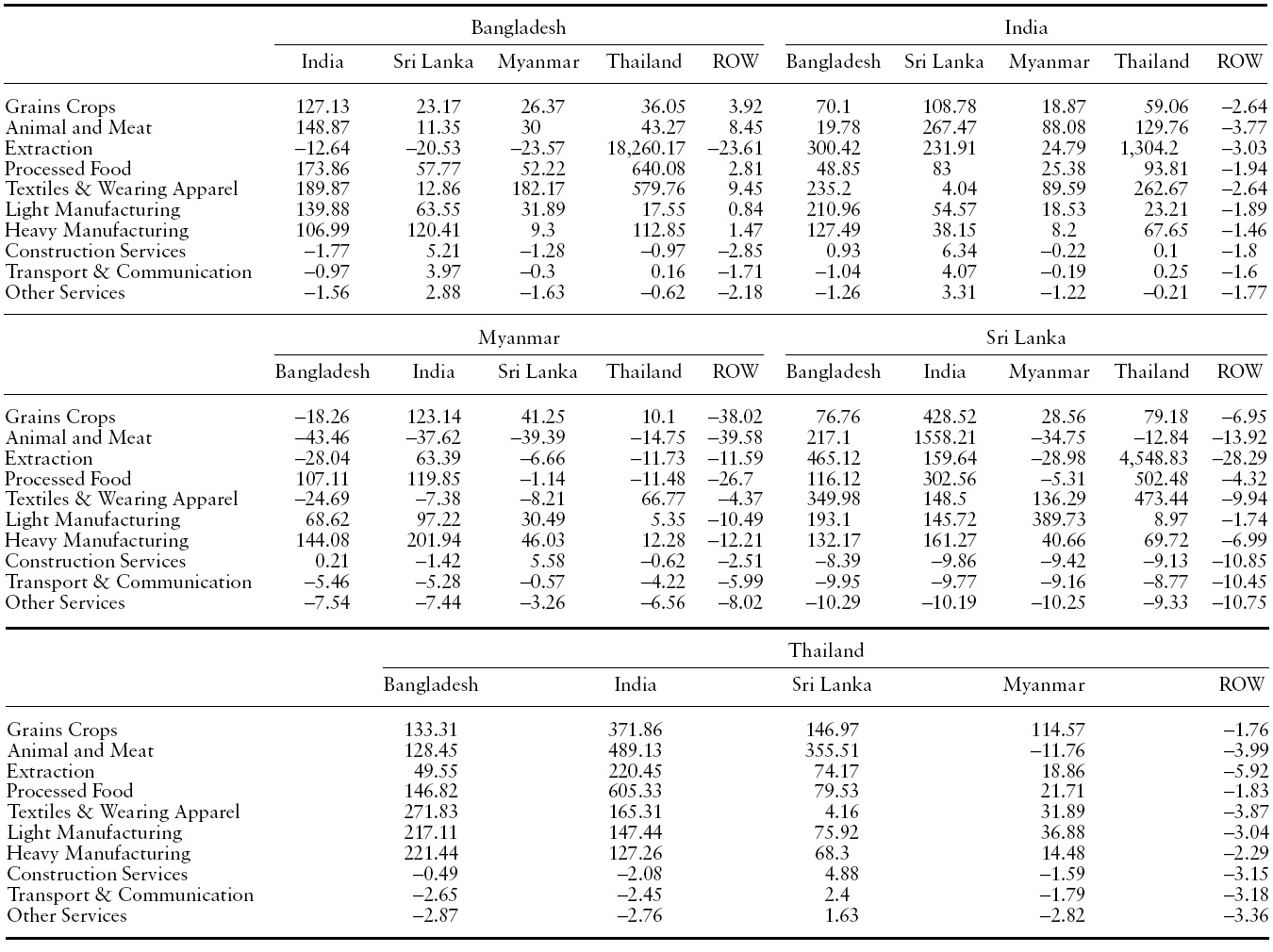
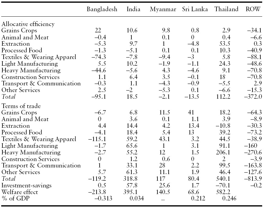
[Table 5.] Commodity decomposition of welfare effects (US$ million)
Commodity decomposition of welfare effects (US$ million)
The changes of relative prices of both outputs and inputs due to trade liberalisation within BIMSTEC will be transmitted to the industries and input markets of the members as well as the other trading partners. A robust analysis of the possible welfare consequences of BIMSTEC FTA requires the contextualisation of interactions among different sectors of the group. Partial equilibrium analysis has the advantages of analytical simplicity and the capability of using disaggregated data, whereas the GTAP model allow these changes within and between sectors in the output mix and factor demands.
The money-metric decomposition of the welfare effect in the standard GTAP model of BIMSTEC FTA is portrayed in Table 5. The simulation is carried out after aggregating the data of 57 sectors into 10 broad sectors.14 The net welfare effect is the sum of allocative efficiency, terms of trade and I-S effects, which is US$972.6 million in BIMSTEC. The results demonstrate that Bangladesh is a net loser in forming BIMSTEC FTA, by US$ 213.8 million fromfull tariff elimination. The other countries derive net welfare gain from the preferential liberalisation, although the amount varies depending on the extent of various effects. Thailand derives the highest net gain, which is US$582.2 million, followed by India, Sri Lanka and Myanmar. The welfare gain for Thailand is due largely to allocative efficiency improvements. For Bangladesh, the overallwelfare impacts are negative, much of which can be attributed to adverse terms of trade effects.
Among the BIMSTEC members, only Bangladesh incurs terms of trade loss, which is significant. The order of terms of trade gain for the other countries is the same as the net welfare gain. The results of SMART simulation demonstrate positive terms of trade gains for all the BIMSTEC members for the estimated export elasticity, gains that vary little for different elasticity values. The I-S effect is negative for Thailand and Bangladesh. Thailand and India derive allocative efficiency gains while the other members reveal losses.
The results are similar to those of Strutt (2008) who conducts simulations of BIMSTEC FTA based on database version 6 in a recursive dynamic model projected for the year 2020. In Gilbert (2008), Bangladesh and Sri Lanka incur a welfare loss of US$126.9 million and US$14.1 million, respectively. However, the amount is larger for Bangladesh,while Sri Lanka derives hugewelfare gains in the present study. Strutt (2008) reveals a net welfare loss for Bangladesh, amounting to US$267 million, which includes losses of terms of trade, capital and equity; although a meagre gain of allocative efficiency (US$3 million) is included in the net welfare effect. The other countries derive significant welfare gains from full tariff elimination within the bloc. This indicates that BIMSTEC FTA is beneficial for the members except Bangladesh although there is a possibility of small efficiency gains for the country in the long run, when all the sectors of the economy are taken into account.
Commodity decomposition of the allocative efficiency effect helps identify the sectors that incur losses and that pull off gains. The results indicate that six broad sectors out of ten end up with losses. Bangladesh incurs huge allocative efficiency loss in the textiles and wearing apparel sector, which is followed by the heavy manufacturing sector. Indeed, the textiles sector is the major strength of the Bangladesh economy, earning more than three quarters of its export receipts and employing around 2 million workers. A substantial loss in this sector implies devastating consequence of the FTA on the economy. Conversely, grain crops achieve notable gains, followed by light manufacturing and some other sectors. But these cannot offset the losses, and the country ends up with significant allocative efficiency loss. India, Sri Lanka and Myanmar also go down in textiles but these are minuscule compared with that of Bangladesh.
On the whole, Myanmar and Sri Lanka incur some losses and India attains some gains. Thailand derives gains in almost all the sectors and substantial gains in the processed food and light manufacturing sectors. Among the BIMSTEC members, Thailand derives the highest allocative efficiency gains.
Terms of trade decomposition suggest that Bangladesh would experience even more adverse consequences in the textiles and apparel sector. Crops, processed food and manufacturing are the other sectors that would be negatively affected, but the impact on heavy manufacturing would not be that adverse compared with the allocative efficiency loss in that sector. The other members would derive a significant terms of trade gain in most of the sectors.Anegative effect is observed inThailand’s extraction sector.The rest of theworldwould incur loss in allocative efficiency in almost all the sectors, with a very small gain in extraction and transport sectors. However, its loss of terms of trade would take place in all the sectors.
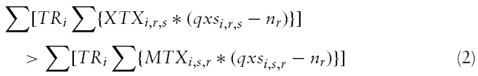
The loss of allocative efficiency due to BIMSTEC FTA is contradictory with the theory, as the tariff elimination is supposed to bring about a positive efficiency effect. However, the negative aggregate as well as sectoral efficiency loss can be explained by the magnitude and interaction of the pre-existing sectoral subsidies with the quantity change in imports and exports after the removal of import duties within the bloc. The sign of the effect would depend on whether the quantity change in exports that receive domestic subsidies surpasses the effect in quantity change in imports due to the removal of tariff liberalisation. Specifically, following the derivation of decomposition of themulti-region
where
Bangladesh’s allocative efficiency loss of over US$95 million could be caused by the pre-existing trade protection in the economy, most of which is accounted for by the textiles and wearing appeal sector (Table 5). It can be argued that the substantial output subsidy provided in this sector leads to this loss since the BIMSTEC FTA requires only the tariff removal, not the elimination of subsidy to export-oriented sectors.15 Therefore, the increase in exports and the decrease in imports through equation (2) would provide negative estimates for the allocative efficiency effects related to exports and imports, provided that the export subsidy rate and quantity of exports are large relative to the import tax rate and quantity of imports. Thus, the loss of allocative efficiency can be attributed to the structure of subsidies prevailing in Bangladesh, Myanmar and Sri Lanka, which leads to a higher performance of exports than that of imports, thereby providing an overall negative effect.
The country level changes in sector-wise exports are interesting (Table 6). Bangladesh’s exports to Sri Lanka and Thailand would increase in most of the sectors, and the majority of the sectors would increase exports to India and Myanmar.The textiles and apparel sector,whichwould face substantial allocative efficiency and terms of trade loss, would experience notable increase in exports except to Sri Lanka. Exports of heavy manufacturingwould also increase substantially except to Myanmar. Overall, BIMSTEC FTA would open up a significant export market for Bangladesh in India and a reasonably prospective market in the other countries.
[Table 6.] Changes in intra-BIMSTEC exports (percent)

Changes in intra-BIMSTEC exports (percent)
India’s exports to Sri Lanka would increase in all the sectors, but decrease marginally in a few sectors, such as construction, transport and other services, to Myanmar, Bangladesh and Thailand. Its extraction exports are likely to increase substantially to Bangladesh, Sri Lanka and Thailand, and exports of textile products would rise significantly to Bangladesh, Myanmar and Thailand. Conversely, Myanmar’s exports to Bangladesh demonstrate a notable reduction in the sectors that include agriculture, extraction, textiles, manufacturing and services. Its exports to India and Sri Lanka would also decrease in five to six sectors but a significant loss would take place in livestock. Exports of only two sectors, light and heavy manufacturing, would increase to all the countries, with a significant proportion to Bangladesh and India. Sri Lanka would incur an insignificant loss of exports to Bangladesh and India in service sectors. In addition to these sectors, the loss of exports to Thailand would extend to livestock. The country’s notable decrease in exports to Myanmar would take place in the livestock and extraction sectors. On the other hand, Thailand would have with meagre losses in exports to Bangladesh and India in services, to Myanmar in services and livestock, and to Sri Lanka in no sectors.
In general, Thailand appears to be the most promising export market for Bangladesh, India and Sri Lanka, especially for potentially spectacular growth in exports of extraction. These countries are also potentially good export markets for Thailand; that is, the possible gains are of both the ways. Thailand has good prospects in grain exports to Myanmar and has the possibility to expand exports in extraction and manufacturing.Myanmar also has good prospects in enhancing exports in processed food and manufacturing to Bangladesh, and in grains and extraction, in addition to these two sectors to India. Its textiles sector has a good prospect in the Thai market. Excluding Bangladesh, the countries would also incur loss in exports to the rest of the world in all the sectors. The losses would be very small for Thailand and India in all the sectors, but significant in grains, crops and meat forMyanmar and extraction for Sri Lanka. Bangladesh’s exports of extraction sector would also be affected significantly.
Finally, the results can be compared with those of the other two studies conducted in the context of BIMSTEC. In Strutt (2008), the net welfare effect of all BIMSTEC members is higher than that of the present study, with a higher negative net welfare effect for Bangladesh. This is perhaps because it includes Japan, one of the biggest economies in the world, in the FTA, and reports the cumulative effect of 11 years in the simulation. In Gilbert (2008), the result is a bit different, with net welfare loss for both Bangladesh and Sri Lanka, but the result is almost similar to the present study. However, this study exclusively focuses on BIMSTEC as well as examines the effect of BIMSTEC FTA on Myanmar, which is an improvement over the previous studies that exclude this important member.
7Pesaran and Shin (1999) show that both FMPH-OLS and ARDL estimators are applicable in small sample (even for n = 20). However, based on Schwarz Criterion (SC) ARDL performs better than FMPH-OLS. As they notice, ‘The ARDL-SC procedure when combined with the Δ-method of computing the standard errors of the long-run parameters generally dominates the Phillips-Hansen estimator in small samples. This is in particular true of the size-power performance of the tests on the long-run parameter’ (Pesaran & Shin, 1999, p. 374). 8The results of the tests are not reported in the paper. However, these can be made available upon e-mail request to the corresponding author. 9The bounds test is a simple F-test to determine the joint significance of the lagged variables. 10The explanatory variables have not been found to be cointegrated for any of the BIMSTEC countries, which meets the requirement of the FMPH-OLS (Pesaran & Pesaran, 1997). 11The full results can be made available upon request. 12By definition, the terms of trade effect is the effect of a tariff on the relative price of a country’s exports on world market compared with its imports. When a large country imposes a tariff, it causes a reduction of import demand and thus reduces the price of the imported goods relative to its exports, and improves its terms of trade. 13Panagariya (1999a) also argues that ROOs may counteract trade diversion. By stepping ahead, Duttagupta and Panagariya (2007) demonstrate that ROOs can improve the political viability of FTAs. 14The base year of the data is 2004. See, Narayan and Walmsley (2008) for details on the database. 15In theGTAP database, the subsidy variables for BIMSTEC countries are: (i) percentage ad valorem rate of output subsidies in region r; (ii) percentage ad valorem rate of export subsidies; (iii) MFA export subsidy equivalent; (iv) ordinary export subsidy; and (v) ordinary output subsidy.
The present paper adopts partial equilibrium andCGEmodels to analyse the possible trade,welfare and revenue effects of a preferential liberalisation in BIMSTEC through forming an FTA within the bloc. The SMART model is a widely used single market simulation tool to analyze Vinerian effects of FTAs. The major limitation of the model is that it assumes infinite price elasticity of exports, although some recent studies confirmthe value to be around one. Therefore, export elasticity has been estimated for the countries by adopting FMPH-OLS and the ARDL models. The likely trade effects are calculated based on various estimated elasticity values as well as with infinite elasticity to comprehend a range of the effects of BIMSTEC FTA.
The results of SMART model demonstrate that there is a high trade potential even for comparatively price-inelastic export supply function, which means that trade and welfare gains might be even higher for BIMSTEC countries. The analysis indicates that the trade effects would be higher for the bigger economies, although the losers would be smaller countries in terms of revenue loss. This has a powerful policy implication for proper design of the compensation mechanism and technical support for the smaller economies so as to offset negative effects. Based on the standard GTAP model, the CGE analysis reveals that Bangladesh is the only member that would incur a net welfare loss by joining the BIMSTEC FTA.The paper also tries to explain the negative allocative efficiency effect,which is absent in the existing literature. Sector-specific allocative efficiency and terms of trade losses are also observed,which include Bangladesh’s substantial loss in its textiles and wearing apparel sector. The real outcome would, however, depend on the trajectory of the liberalisation and investment promotion within the scheme, aswell as the future dynamics of the regional and global economy. Since the bloc’s welfare effect is positive in the GTAP analysis, and trade and welfare effects are positive in SMART analysis, an FTAwould bring about an overall positive impact on the bloc with some country-specific adverse effects.