The recent debate on globalization, particularly trade liberalization, seems to have reached every corner of theworld. In theory, the consensus that trade liberalization benefits every participant in international trade has not been fully substantiated, especially for participants too far from market centers and too small to compete (Stiglitz, 2004; Chang, 2003). The arguments on whether the poor benefit from trade liberalization are even more controversial given the limited information available to substantiate most of the claimed gains. Trade theories – Richardo’s comparative advantage and Heckscher-Ohlin’s (HO) factor proportion – show that trade benefits all countries who participate under the specified assumptions. These theories do not answer the specific questions about whether the poor in each country benefit. The Heckscher-Ohlin theory identifies winners and losers based on who owns what in each country. However, the assumptions in the H-O theory are too general to point out the gains to the poorwhose access to resources, other than their own labor, is limited.
Most previous empirical studies that deal with the implications of trade liberalization are undertaken in Asia, and Latin America. Similar studies on African economies are very scanty, but growing as the voices of the poor become louder. The reports coming from countries in Asia show some consensus, in that trade liberalization has positive effects even for poor families. Studies from Latin America, although not as strong as those fromAsia, also indicate promises of similar trends (Cline, 2004). For the case of African economies, the limited empirical findings report conflicting results. Hence, it is timely and important to undertake such a study for cases that represent Africa to fill the empirical gap and to answer the question of how trade liberalization affects those rural farm households far from the center and from the media.
Ethiopia has undertaken several policy reforms since 1992. One of the crucial policy reforms relevant for rural economy was devaluation of the birr (Ethiopian currency) in 1992. The direct impact of the devaluation would be for farmers to get better prices for their export crops, such as coffee and chat.1 Since more than 90% of coffee production comes from small-farm holders (Dercon, 2002), it is expected that farmers would be the direct beneficiaries of currency devaluation. The country also embarked on dismantling quantitative restrictions and gradually reducing the level and dispersion of tariff rates. As a result of the reform, tariff rates narrowed down from 0–240% to 0–80% in 1995 and then to 0–35% in 2002 (World Bank, 2004). Duties on all exports,2 other than coffee, were lifted in early 1990s. The coffee export duties were unified and set at 6.5%. One expects that most of the policy changes would promote export of not only traditional cash crops but also food crops often traded only locally (such as teff,3 wheat, barley, and maize) and the benefit trickles down to most farm families in rural Ethiopia. In 2008, Ethiopia launched the Ethiopian Commodity Exchange (ECX) marketplace to provide market integrity and to enhance market efficiency through rural electronic price ticker system. So far the ECX has been providing its services for major food crops, although recently it has added coffee to its system. In a country where rural employment opportunities are limited or only serve as a last resort survival strategy (Lemi, 2009), the role of change in crop prices are critical. It is with this backdrop that this study plans to assess the role of trade liberalization on poverty in rural Ethiopia.
The basic question asked in this study iswhat determines change in poverty status of households in rural Ethiopia. Among the many factors, the study focuses on the role of economic reform in general, and trade liberalization in particular, in influencing escape from poverty. The results of the study are expected to provide answers to the following questions: what happened to poverty when the government-implemented reform programs too slowly (but surely) open up its markets to the world? Which household characteristics and trade policy factors help families to benefit from trade policy reform to escape poverty? The purpose of this study is, therefore, to undertake empirical study on the impacts of trade liberalization on changes in poverty status using rural household survey data from Ethiopia.
The remaining parts of the paper are organized as follows. The next section presents a review of previous studies and discussion of Ethiopia’s experience in trade liberalization. The third section presents data and methodology followed by discussion of the results. The final section provides conclusions with policy implications.
1Stimulant leaf often exported to the Middle East and other parts of Africa. 2The major agricultural and related export items are coffee, chat, oilseeds, pulses, livestock, and livestock products. 3Teff is a tiny cereal grain native to the African country of Ethiopia. It is one of the staple food items in the country and used to make a pancake-like bread.
Following the predications of trade theories, Bhagwati and Srinivasan (2002) and Dollar and Kraay (2004) argue that trade liberalization helps reduce poverty through growth, especially in developing countries. Harrison et al. (2003, 2004) present empirical results in line with the above argument and contend that the poor gain from trade liberalization in, respectively, Turkey and Brazil. Others, however, argue that the effect of trade liberalization is not enough and is not straightforward to benefit the poor in developing countries (Carneiro&Arbache, 2003), or has only mild aggregate welfare gains (Vos & Jong, 2003). The negative effects of trade liberalization on poverty are also reported in recent studies (Annabi et al., 2005; Cororaton, et al., 2005; Sharma, 2005). In developing countries, the role of shocks on poverty and the poor is often emphasized in addition to the role of economic reforms and growth (see Dercon, 2002; and Dercon et al., 2005 for Ethiopia; McCulloch&Calandrino, 2003 for China; Appleton, 2001 for Uganda; Fofack et al., 2001 for Burkina Faso; and Ocran et al., 2006 for Ghana). Several recent studies have documented detailed reviews of the literature on the relationship between trade liberalization and poverty (for instance, see Winters, 2002; McCulloch et al., 2001; Winters et al., 2004; Cline, 2004).
Theoretically, one also needs to look into the smallest unit of analysis (in this case a household), not just macro level results, to investigate the micro level impacts of policy changes. Dercon (2006) looked into a standard household model under perfect market assumptions to show how household utility function would be affected by a change in output and input prices.4 The first-order condition of a typical household utility maximization results in the following:
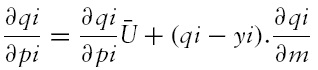
where
Previous studies identified several factors that need to be considered to examine the impacts of trade liberalization on a community or a region. Winters (2002) identified six variables that potentially affect the link between trade, trade policy, and poverty. The four factors that are relevant for the case of farmers in a rural setting are: the price and availability of goods, factor prices (i.e., income and employment), government’s transfers influenced by changes in trade taxes, and external shocks (in particular, changes in the terms of trade). In poor developing countries, the extent of the impact of each of these variables differs depending on the degree of access to markets and the degree of institutional support available to farmers.The intricacy of the impacts of these factors makes it difficult to pinpoint to the exact effects on groups affected by trade reform.
That led Winters et al. (2004) to conclude that given the variety of factors to be considered, lack of consensus on the effects of liberalization on the poor and poverty is not surprising. They argue that simple generalization on the effects of trade on the poor and about all countries will just be wrong. Considering the living conditions of the poor and their mobility to look for better income or living conditions, Coxhead (2003) argues that rigorous answers to the effects of liberalization on poverty have proved elusive. The lack of consensus leaves policy makers to look for micro level information on the effects of liberalization in a given region and/or on a given group in a country. This warrants the need to look into individual countries, and perhaps communities, to understand the peculiar circumstances that make them respond differently to different reform measures.
The results of most of the studies, which have used different methodologies, are mixed. The studies that report pro-poor effects of trade reform often qualify their findings with other necessary conditions. Studies by Ocran et al. (2006), Fofack et al. (2001), and Son and Kakwani (2006) conclude that, on average, liberalization favors non-poor in their sample countries, whereas Dercon (2002, 2004), and McCulloch and Calandrino (2003) show that growth, or related trade policy reforms, is pro-poor, for their sample countries and periods of study. Dercon (2002, 2006) and Ocran et al. (2006) reported results from empirical analysis that examined the impacts of economic reform on poverty using household survey data from Africa. More importantly, both studies incorporate specific trade reform variables in their regression analysis to examine impacts on poverty or the poor. Dercon’s (2002, 2006) studies used a dataset from Ethiopia,5 whereas Ocran et al. (2006) used a similar dataset from Ghana. However, they followed different estimation approaches. Ocran et al. (2006) used limited dependent variable estimators since income and consumption of farmers in their sample were not observed. They simply grouped their sample farmers into those who had produced cash crops and those who did not produce cash crops during their study period.
Dercon (2002, 2006) used consumption expenditure data to assess the impacts of economic reform on consumption of the poor and hence the change in poverty status. Dercon (2006) looked at the determinants of change in consumption for poor families using a smaller sample (only six of the 15 survey sites) between 1989 and 1994. Dercon reported that land, terms of trade (producers’ price index and consumers’ price index), rain shock, and road infrastructure are positive and significant determinants of change in consumption between the two survey years. The terms of trade variable is the key variable that captures economic reform for rural households in Dercon’s study. This key variable is the weighted sum of the prices of traded crops in each survey site. As such it only reflects a crude economic reform measure, not trade policy reform, for some households who cultivate and consume only some crops out of the many crops produced and traded in the market. The study concluded that economic reform programs do not deliver similar benefits to the poor and further indicated that if there had been no reform, poverty would have increased in 1994.
There are other studies that analyzed poverty dynamics and transition in Ethiopia using the more representative dataset (Kebede et al., 2005; Bigsten et al., 2003; Bigsten&Shimeles, 2008) and identified relevant correlates. Although these studies focused on the determinants of poverty transition and dynamics in rural Ethiopia, none of them analyzed the direct impacts of trade liberalization. Bigsten et al. (2003) have used similar datasets and methodologies to the present study. However, the only variable that they have incorporated in their estimation is type of crops (including chat, coffee, and teff) as a dummy variable for those households who produced any of these crops. As such, this variable does not take into account change in prices or any direct liberalization variable. Their results show that chat-producing poor households had a higher chance of falling in to poverty, and chat-producing non-poor households in 1994 had a lower probability of falling into poverty. Can we get a similar pro-poor effect for chat-producing households if we use actual price changes between 1994 and 1997?
Similar to Dercon’s (2006) and Bigsten et al.’s (2003) approaches, the present study estimates change in poverty status equations augmented by trade reform variables to generate relevant coefficients to confirmor reject the pro-poor results of previous studies in the context of Ethiopia. The present study differs from that of Dercon’s (2006) in three ways. First, the present study uses a larger representative sample (1400 households as opposed to 354 poor households). Second, we estimate the determinants of change in poverty status, not just change in consumption for the poor, for those households who escaped poverty, fell into poverty, and remained poor during the study periods. Third and most important, this study estimates the impact of trade liberalization through changes in prices of six major crops (both cash and food crops) unlike the composite terms of trade variable employed in Dercon (2006). This study also differs from Bigsten et al. (2003) since the present study includes actual changes in prices of the major crops, as opposed to dummy variables for the types of crops produced, as was the case in Bigsten et al. (2003).
4Note that this simplistic model is presented only to fix ideas for discussion, not to generate reduced equations for estimation. 5Dercon’s studies used data from 1989 and 1994 survey years and for only six of the 15 survey sites. These sites were selected as drought-prone areas and may not be representative of the farming community of the country.
The Department of Economics at Addis Ababa University, in collaboration with various international research institutions, has been gathering socio-economic data from 1500 representative farm households from 15 survey sites in Ethiopia since 1994. In 2000, the survey was in its sixth round (although not on a regular interval); the same householdswere interviewed to obtain information on various modules. The core modules that appear on the questionnaire are information on demographics, assets, farm inputs, farm outputs, consumption, livestock, and health. The 15 survey sites are scatted across four regions (Amhara, Oromia, SNNP,6 and Tigray) of the country, representing different farming systems, with the exception of pastoral areas.
This study has used datasets from two of the six rounds7 (i.e. 1994 and 1997) to investigate the effects of trade policy reform. The selected survey years (1994–1997) are periods during which the country adopted significant economic policy reforms and structural adjustment programs. Since the data have been collected from the same households for all the rounds (with very low attrition rate),8 it is suitable to analyze the impacts of policy reforms on the sample households over time.
As indicated above, there are several policy reformvariables, including changes in prices of inputs and outputs and prices of inputs that affect the level of poverty in a country. In this study, we will use the change in prices of the major crops in Ethiopia as indicators for trade policy reform. In addition to the two major export crops (i.e. chat and coffee),we also include changes in prices of other major staple food crops produced in Ethiopia, namely, teff, wheat, barley, and maize. For input prices, we will use change in the cost (price) of one of the major farm inputs that farmers use: fertilizer. Almost all fertilizer types used in the country are imported and the effect of trade liberalization can affect farmers’ income or consumption. The other input that farmers use on their farm is pesticide, which is also affected by trade policy reforms.However, the use of pesticide is not widespread compared to that of fertilizer use among farmers with small land holdings. Hence, we will use the price of fertilizer at the nearest district market to calculate the relative prices of the major crops to examine its impact on poverty status.
The debate over whether income, consumption, or asset provides better information for the study of poverty dynamics is still not yet settled. There are those who favor consumption (Dercon, 2002) for its reliability and completeness since it captures actually spent expenses. While others favor income as a measure of poverty dynamics since it reflects not only consumption but also income growth that has been saved or invested to build assets (Nicita, 2004). Still others argue that assets should be the key indicator of poverty status since it is stable and also includes both private and public assets to supplement other money-metric indicators (Booysen et al., 2008). The present study argues that poverty dynamics, in the context of the survey data used in this study, is better reflected using consumption data mainly due to understatement of income and longer recall period used to gather income data compared to consumption data. Once the issue of yardstick is settled, the next step is to construct poverty lines at the country, region or village levels. The next section sheds some light on the construction of poverty lines for the two survey years used in the present study.
One of the cornerstones of poverty analysis is the computation of a poverty line for a country or a region under investigation. Ravallion (1998) defined a poverty line as a monetary cost to a given person, at a given place and time, of a reference level of welfare. People who do not attain that level of welfare are deemed poor. Others define that a poverty line measures the minimum income or consumption expenditure or asset required to attain basic daily activities for a person. Although it sounds simple in the definition, there are serious disagreements onwhat the daily activities include, whether income, expenditure or asset should be the yardstick, and howto adjust the poverty line over space and time (Ravallion, 1994; Ravallion & Bidani, 1994). Recent studies argue that these concerns are not easy to resolve especially in the time of a rapidly changing world (Osberg & Xu, 2008) and at a time when the relevance of previously ignored poverty dimensions come to light (Alkire, 2007).
Despite the call for locality specific poverty lines, the World Bank’s attempt to come up with an international poverty line for entire developing countries is criticized as overly simplistic.9 For instance, if one adopts the $1 or $1.25 per day per person income poverty line of the World Bank, one would find an overstatement of poverty rate (perhaps close to 60–75%) in Ethiopia. As a result, most studies in developing countries use survey data to come up with national poverty line and/or locality specific poverty lines in a country. Osberg and Xu (2008) show that, for the case of China, the commonly accepted international poverty line defined as one half median national equivalent income is becoming increasingly relevant for a changing world.
For the case of Ethiopia, there are several studies, that the author is aware of, that computed poverty lines using the same dataset used in the present study. Dercon and Krishnan (1998), Dercon (2006), and Bigsten et al. (2003), Kebede et al. (2005) and Bigsten and Shimeles (2008) have computed poverty lines for rural and urban10 (only the latter two studies) Ethiopia. They have used a Cost of Basic Needs (CBN) approach to arrive at the computed poverty lines for each of the survey sites under study. Dercon and Krishnan (1998) arrived at the average poverty line of 528 birr per person for 1994 where as Kebede et al. (2005) arrived at 726 birr per person for 1995 using the same data and similar methods. The Welfare Monitoring Unit (WMU) of MOFED11 (2002) Ethiopia also came up with 1073 birr per person for 1995 for rural Ethiopia using other survey datasets. If we go by the World Bank’s $1 per day per person poverty line, the comparable annual poverty line for Ethiopia would be 2190 birr (at 1995 exchange rate of $1 = 6 birr) per person for 1995. The differences in the poverty lines are mainly due to the food basket selected in each case to measure the cost of basic needs, the year under investigation, and the different survey data used in each study.
Using Foster, Greer, and Thorbecke (1984), the internally computed poverty lines are 380.2 birr per adult in 1994 and 466.6 birr per adult in 1997 for the 15 survey sites in this study. Dercon and Krishnan’s (1998) estimate of poverty line for the year 1994 fits best for the analysis in this study, given that they have used the same survey data from 1994 and a representative food basket. I have adopted the site-specific poverty lines reported in their study.
Although some of the above studies analyzed poverty dynamics, it is not clear how they arrived at the consumption poverty line for the subsequent years. Some studies (for instance, Dercon & Krishnan, 1998; Bigsten et al., 2003; Bigsten & Shimeles, 2008) have used either the poverty line of the base year as deflator or price index of local products to update base year poverty lines. In this study, the national food price index is used to calculate the real consumption expenditure for 1997 to arrive at the consumption poverty line in 1997. It is important to also note that in year 1997 national consumer prices (and food prices) were below that of 1994, hence 1997 values were deflated using national consumer price index. Since farm households purchase nationally traded goods (such as salt, oil, kerosene, clothing, school and medical supplies, and so on), their consumption should be deflated by national price index, not just local prices of food items.
[Table 1.] Poverty status change between 1994 and 1997
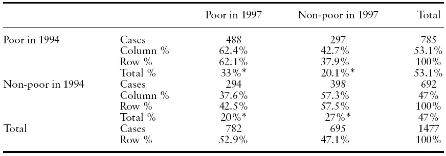
Poverty status change between 1994 and 1997
Table 1 reports changes in poverty rate between 1994 and 1997 using sitespecific consumption poverty lines discussed above. Over 62% of households who were below the poverty line in 1994 remained poor in 1997. Out of those householdswhowere above the poverty line in 1994, close to 43% fell into poverty in 1997. The overall poverty rate for the country was about 53% both in 1994 and 1997. These numbers refer to households in the rural part of the country. As reported in MOFED (2002), the poverty rate could be lower if one takes into account urban households as well. For instance, MOFED (2002) reported that in 1995/96, the national poverty rate was 45.5%, with a higher rural poverty rate (47%) than urban (33%). However, MOFED and the other studies have used different methodologies and datasets to arrive at the poverty lines and hence comparison may be unwarranted.
The aim of this study is to answer the questions: what factors kept 488 households poor both in 1994 and 1997? What factors kept 398 households above the poverty line in both years? And finallywhat pushed 297 households out of poverty and 294 households into poverty in 1997? One common theme of all of these questions is to specifically analyze the role of trade liberalization in influencing these poverty status dynamics.
3.2 Multinomial Logit (MNL) and Relative Risk Ratio
Recent studies that investigate the role of trade liberalization rely on Computable General Equilibrium (CGE) models to compute relevant impact coefficients (Hertel et al., 2003).12 However, for the case of Africa, where available data do not allow one to build broad-based CGE models, many studies resort to partial equilibrium analysis to address welfare effects of reforms (Ravallion, 1989; Dercon, 2002; Porto 2003), as a result Partial Equilibrium analysis is emerging as an alternative to General Equilibrium Models (McCulloch & Yiying, 2003; Niimi et al., 2003; Litchfield et al., 2003). It has also become common practice to model poverty status of households using multinomial logit model. The Multinomial Logit model estimates the probability of being in a particular poverty state out of several unordered alternatives (Niimi et al., 2003).13
The probability that household
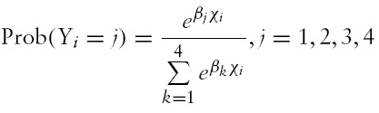
where
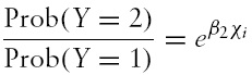
This paper reports the impact of each explanatory variable on the relative risk ratios (RRR) rather than the actual coefficients, which gives us the odds-ratio. The relative risk ratios are the ratio of the probability of each outcome relative to the probability of the base category. If we set

where
One of the concerns with the estimation ofMNLis the assumption of independence of irrelevant alternatives (IIA). If this assumption is violated, the estimators from MNL are not valid. The author has conducted the Hausman test to check whether the MNL models estimated violate the IIA assumption. The Hausman test is performed for all specification and by omitting (i.e. using as a base) all the categories one at a time. In almost all cases, the Hausman chi-square is 0.01 for all specifications where category 4 (being non-poor in both years) is used as the base outcome, which supports the IIA assumption to estimate the multinomial logit model. It is only when category 3 (i.e. falling into poverty) is used as a base outcome that the Hausman test rejects the IIA assumption. However, as stated above, category 3 has not been used as the base outcome in any of the results reported here. Hence, the Hausman test validates the results reported from the multinomial logit specifications.15
To show robustness of the results, standard probit model and random effects logit models are estimated. Results from the probit model are reported in the Appendix (Tables 1A–3A). The probit estimation results address the concern over the IIA assumption often raised with the MNL estimation. As can be seen below, the results from the probit, random effects logit aswell as theMNLmodels are similar. In fact, for the key variables that motivate this study, the results from theMNLmodels are stronger than the results from the probit and random effects logit models.Of course it is not reasonable to compare these results from different estimation specifications. This is because the results from MNL reports relative risk ratio (RRR) of all alternatives compared with the base alternative, whereas the probit and the logit models report only the original marginal effects. Still, the same insight can be drawn fromthe three specifications. This confirms that MNL model fits the data well compared with the simplistic probit and logit models.
3.3 Correlates of Poverty Dynamics
To answer the questions poised from the outset, this study estimated the multinomial logit model with the relevant correlates that affect poverty status. The right-hand side variables are divided into three groups: demographic composition, assets and inputs,16 and trade policy reform variables. I have used variables from the survey data to approximate each of these categories. For some of the variables, which show no or little changes during the two survey years, I have used the 1994 values of these variables to examine the impact of initial conditions on the poverty status of households.
Bigsten et al. (2003) have also used a multinomial logit model to estimate the determinants of poverty status in rural Ethiopia. In their study, and in Kebede et al. (2005), poverty status changeswere regressed on initial (1994) socioeconomic characteristics of households to determine factors that had a significant impact on change in poverty status. However, they haven’t looked at the specific role of trade liberalization. To fill this gap, I augmented their model using changes in trade policy variables identified in Dercon (2006). In addition to the initial conditions (1994) used in previous studies, I augmented the poverty status model by changes in the real and the relative prices of major crops. The variables in the right-hand side of the estimated equations are discussed below.
Previous studies identified three key correlates of poverty and poverty dynamics, namely, demographic composition and education, asset and agricultural inputs, as well as trade policy reform variables. In agrarian economies like Ethiopia, one of the resources that households have control over is labor. As a result, human capital is the key input in farming and other activities. The composition and the education levels of household members are therefore important to determine the human capital endowment of a household. To account for this, I have used initial values of family size in adult equivalents, age of household head, dummy for female headed households, number of male adults, number of female adults, number of dependants in the family, and number of students below age 15.
For resource-constrained farm households, farm tools, access to credit, and other farm inputs help them to significantly improve their productivity and increase consumption. It is believed that access to these assets and inputs is expected to change poverty status over time. In the present study, the value of major agricultural tools, access to loan, amount of land owned, and the value of livestock owned are key assets that are expected to play a significant role in rural Ethiopia. I expect that the higher the value or access to each of these resources gives households the opportunity to escape poverty or remain above the poverty line.
Two channels throughwhich trade liberalization affects poverty are considered: the price channel and employment channel. Effects through the price channel come either through direct price effects, and/or production effects. Prices of tradable goods are expected to change after liberalization and hence prompt more production of tradable goods. I have used changes in the prices of major food crops (teff, wheat, maize, and barley) and cash crops (chat and coffee) to investigate the implications of these price changes. The changes in prices are in real terms. There may be other price effects through imported input (i.e. fertilizer). Farmers may benefit from an increase in the price of crops that they have sold, at the same time they might also benefit from a reduction in the price of fertilizer as a result of liberalization, as trade theory suggests. To account for the change in relative price effects, I have computed relative prices of each crop (ratio of individual crop prices to cost of fertilizer). Hence, to compare results, the changes in the relative prices of all tradable cropswere also used in addition to the changes in the real prices of each crop. It is expected that for those escaping poverty and those who remained nonpoor, positive and significant coefficients of a relative price imply that households benefit from higher output prices and/or lower fertilizer prices for each particular crop.
There may be households who could not benefit from the price effects due to on-farm consumption of what they have produced. To explicitly account for this, I have controlled for whether households sold part of their products, both in
Descriptive statistics of some of the key variables indicate that the two key resources that seem to partially determine poverty status are the size of land and livestock owned. Those who fell into poverty and those who remained poor in 1997 own less land and less livestock in 1994. The proportion of households who sold at least part of their production increased in 1997 compared with 1994 for all poverty status groups during the main harvest season. This may be an indication of the level of production in 1997 due to relatively suitable weather conditions. As a result of good harvest, almost all prices declined between 1994 and 1997. The exception is the price of chat, which recorded a slight increase for most poverty status groups except for thosewho fell into poverty in 1997. Notice that the prices are in real terms; nominal prices have been increasing since inflation sets in after the introduction of economic reform programs in 1992.
One other pattern to note is the value of coffee production. It is puzzling to see that the increase in coffee production in 1997 is the highest for the two groups (persistently poor and those who fell into poverty) who did worse in terms of poverty status. A similar pattern is observed for the production of barley. It is tempting to conclude from the descriptive statistics that those who increased production of one of the cash crops (i.e. coffee) did not benefit and hence liberalization was
6SNNP stands for Southern Nation and Nationalities People. For the survey the region was divided into three sub-regions (formerly regions 7, 8, and 9). 7These two years are selected for two reasons. First, 1994 and 1997 give us a natural experiment where one can see the effect of both policy and weather shocks. It helps to see how farmers respond when they face these shocks at the same time. Second, the other two survey years in between (1995 and 1996) are too close to the base year (1994) to see any significant response from the farmers. The later years (especially 1999 and 2000) may be ideal to conduct longer panel analysis and they may also introduce other shocks. However, for these years some of the variables that refer to demographics and household composition and related covariates are not consistent with previous year variables and it creates a difficulty to pool the data together from these years. In addition, given the length of time between 1994 and 2000 (and later years for that matter) other significant changes, other than liberalization, might have occurred to influence famers’ response to any price change and hence it creates a difficulty to distinguish responses to policy and other factors set during these periods. 8It is also important to note that the survey was conducted by enumerators by going door-to-door, which makes the response rate so high. 9Some studies use the World Bank’s international poverty line for cross country comparisons (for instance, see Banerjee & Duflo, 2007). 10Gebremedhin & Whelan (2008) also estimated the urban poverty line for Ethiopia; the average poverty line from their estimation is 951 birr per person for 2000. 11Ministry of Finance and Economic Development of Ethiopia. 12For a survey of methodologies used to analyze the impacts of trade liberalization on poverty see Hertel and Jeffery (2005). 13Several studies have adopted a multinomial logit method to study the dynamics of poverty and its determinants (for instance, see Niimi et al., 2003, for China, Bigsten et al., 2003, for Ethiopia and Litchfield et al., 2003, for China). 14Greene (1997) also shows the detailed computation of MNL and indicates the computational difficulty associated with multinomial probit model. 15Alternative methods to the MNL estimation technique would have been Nested Logit (NL) and Duration models. For the dataset used in this study, both methods prove to be inappropriate. NL estimation assumes that choice specific (as opposed to individual specific) information is gathered to estimate the model. Duration models assume that both the start and the end of the poverty spell are known for an individual in the sample, and to do this a longer time period is implied. The dataset used in this study does not have the features required to estimate NL and Duration models. 16In rural part of the country, some assets (such as livestock) are also farm inputs and hence the need to group assets and inputs into one category. 17In almost all specifications, the coefficient of this variable is statistically not significant; as a result the variable has been dropped from estimation equations. 18Given logistic issues during the survey periods, it was difficult to collect the data from all villages at the same time. Hence, there were variations in terms of the months the data were collected. For some villages, the months during which the data were collected fall on the peak harvest season and for others the months fall on the slack season of the year. As the month varies by village, the recall time varies as well, which may result in understatement or overstatement of some values such as income and consumption. To account for the variation in the survey months and hence recall periods, I have introduced the seasonality variable. 19This term is often used in discussion of development in poor countries. The World Bank publications have popularized the term more than any other writings in academic journals. The term pro-poor refers to any policy or targeted programs that directly help the poor (or those below poverty line). In this paper, the term is used to indicate whether the effect of liberalization affects the poor favorably (i.e. pro-poor).
First, it is important to note that some variables that appeared relevant from previous studies became inconsequential in affecting poverty status in the present study. These variables include a dummy for surplus or deficit farmers (Dercon, 2006), a change in employment (proxied by off-farm employment) and, rainfall20 timing and amount. The regression results show that none of these variables matter in influencing change in poverty status. The changes in these factors are either not related to poverty status at all or are not statistically significant to make any difference on the change in the probability of being in a given poverty status. The latter may be the case since there is anecdotal evidence that suggests, in some parts of the country, some of these factors are relevant determinants of change in living standard of farm households.
On the other hand, most village fixed effects are statistically significant in influencing the poverty status outcome of households in these villages.The implication is that there are village specific factors (such as access to markets, infrastructure facilities, etc) that matter more for some villages. Similarly, seasonality had a statistically significant impact. Seasonality is one of the factors that affect poverty status of a family in rural Ethiopia. Issues of seasonality could be within a given year or across years.Given the two major crop seasons (i.e.
In the remainder of this section, I will present results for each poverty status outcome between 1994 and 1997. First, results for the persistently poor (i.e. poor in both years) are presented followed by results for households in transition (i.e. escaped poverty or fall into poverty in 1997).
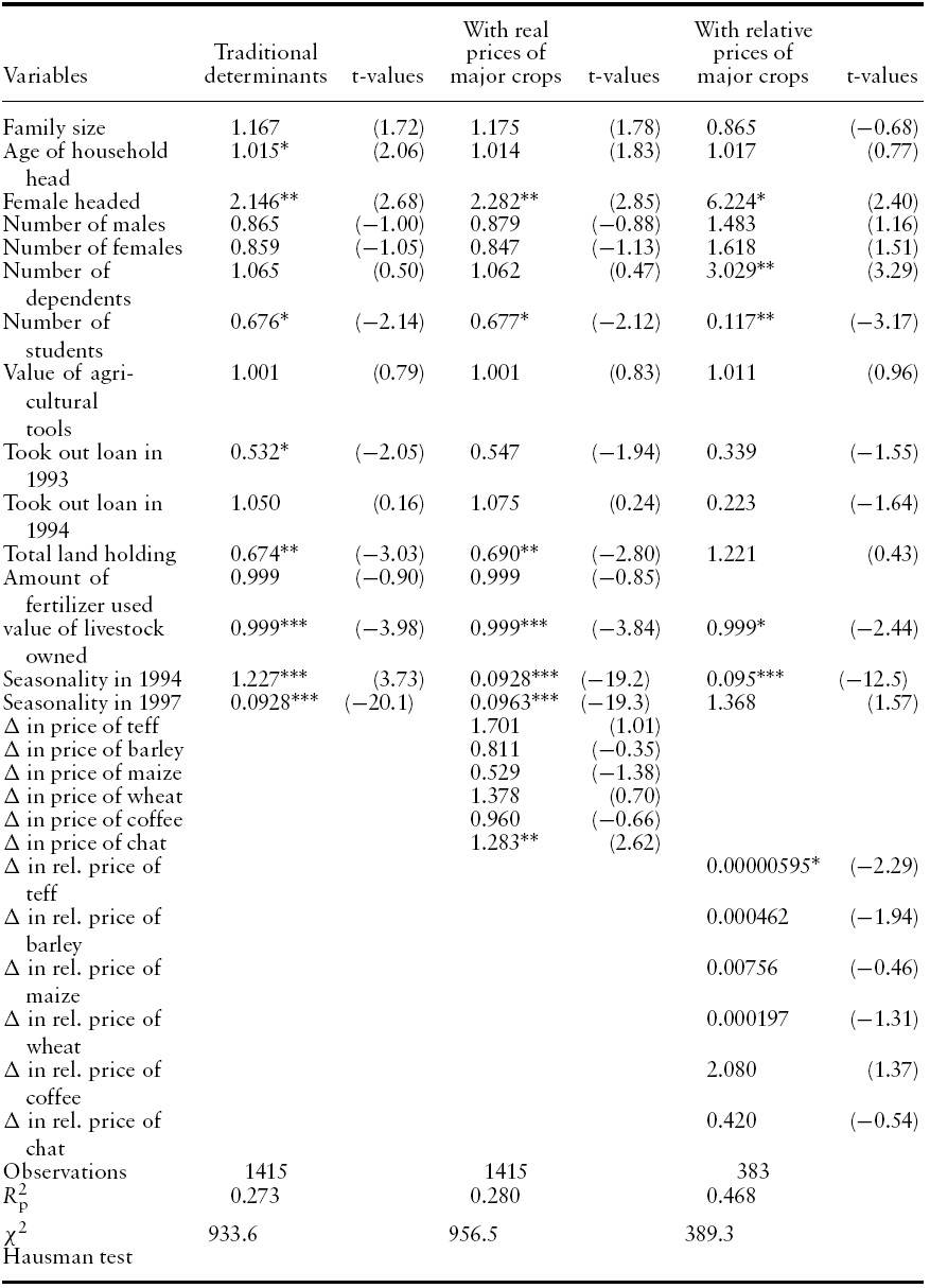
The probability of being persistently poor increases for female-headed households and slightly as the age of the head of the household rises. On the other hand, the probability of being persistently poor decreases for households with a high number of younger students, as well as for those who own large farm land and livestock. Of the market reform variables, change in the price of chat increases the probability of being persistently poor and change in the relative price of teff decreases the probability (Table 2). All other right-side variables are not statistically insignificant. The negative effect of chat price on poverty status seems at odds with the expectation about the impact of liberalization. However, it is important to note that some anecdotal stories seem to substantiate these results. That is, in some part of the country, especially in the eastern part where chat production is dominant, farmers switched from production of food grains to cash crop, such as chat, expecting to receive an attractive price right after trade liberalization (Dercon, 2002). However, in terms of food consumption, the farmers end up purchasing food crops from the market for which the prices were also rising. If the farmers do not receive enough cash from the sale of chat, they end up consuming either less than before or just about the same amount. The perishable nature of chat and the instability in the price of chat in the international market make farmers’ likelihood less stable and hence resulted in no change in their poverty status.
The positive impact of the change in the relative price of teff, which is a staple food in Ethiopia, is not surprising. Teff is one of the most expensive of all the food grains produced in Ethiopia. In fact, the country sometimes exports it to neighboring countries and to as far away places as North America and Europe, although the government imposes restrictions on its export to stabilize domestic market for food grains. As such, those farmers who manage to produce teff, given that they have suitable soil and weather conditions, can improve their livelihood. But what is surprising is that the relative price of teff declined between 1994 and 1997 in
4.2 What Pushed Farm Households into Poverty?
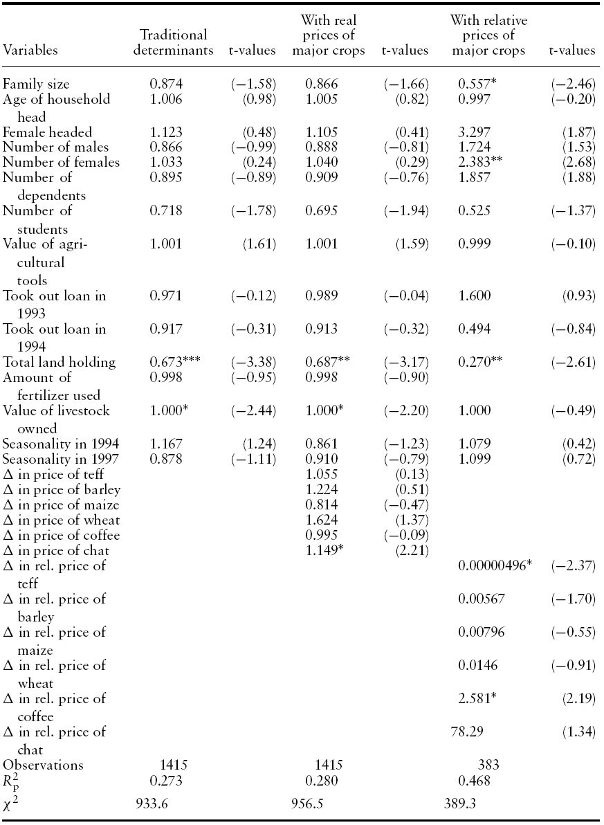
The factors that pushed farmers into poverty are more or less similar to the factors that kept farmers poor. Although demographic and family composition played a relatively smaller role in influencing the probability of falling into poverty, households’ resource endowments played a significant role. The larger the size of farm land owned and the value of livestock owned the lower the probability of falling into poverty in 1997. Among market reform variables, changes in the prices of both cash crops (i.e. coffee and chat) and changes in the relative price of teff also played a statistically significant role. Changes in the price of chat and the relative price of coffee had increased the probability of falling into poverty in 1997, whereas change in the relative price of teff lowered the probability of falling into poverty (Table 3). The story is similar to that of the persistently poor.
Determinant of persistently poor: relative risk ratios (DV: Farmers who remained poor in 1997 with never been below poverty line as a base outcome)
The counter-intuitive negative effects of coffee and chat can be explained by the textbook examples of the problems of exporting primary goods, i.e. unstable prices and limited value added to the raw products due to market imperfections and other natural barriers. The role of the middlemen is equally important in depriving the farmers from receiving their fair share (i.e. reasonable price) compared with the world price for their exports. For instance, from the retail prices of coffee in importing countries, it can easily be shown that the Ethiopian farmers receive only 6–10% of the retail return from the entire value-chain; this compares poorly with, for instance, the Jamaican coffee sector, which receives 45% of the retail return. For the Ethiopian coffee chain, about 39% of the value goes to an intangible return taken by distributors, in addition to the 50–55% distribution margin that goes to distributors. The Ethiopian Commodity Exchange (ECX) marketplace has been launched in 2008 charged with mitigating this problem as one of its objectives.
4.3 How did Farm Households Escape Poverty?
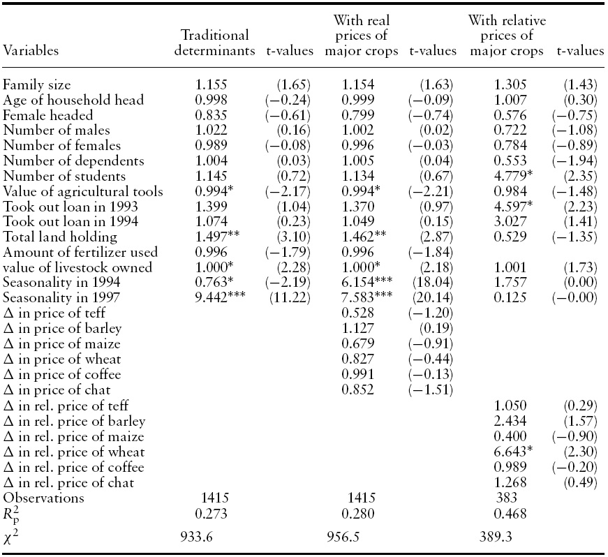
An equally relevant policy question is to knowwhat household characteristics and what other factors helped farmers escape poverty in 1997 and to remain above the poverty line during both years. As evidenced from the results for falling into poverty, family composition did not play a significant role, unlike its negative and significant impact on the households who remained poor during the study years. Size of farmland owned and value of livestock owned, as expected, increased the chances of escaping poverty. Even for these resources, once relative prices of major crops added to the right-hand side of the estimation equation, their significance diminished and instead the number of students, and loan taken out in 1993 became statistically significant. Of the market reform variables, only change in the relative price of wheat increased farm households’ chance to escape poverty (Table 4). The evidence supports the idea that householdswho had access to credit and schooling managed to escape poverty. Families changed their poverty status not due to a change in prices of traditionally exported goods, such as chat and coffee, but as a result of the change in the prices of wheat, which is another major food crop in the country after teff.
It seems that there is a piece of puzzle in the results presented above. Although one expects to see a positive impact of changes in the prices of cash crops, often traded in the world market, to change the poverty status of farm households for good, the evidence shows the opposite. In fact it is the change in the prices of other food crops, teff and wheat that had improved the poverty status of farm households in Ethiopia. As alluded to above, one explanation is that farmers are not receiving the prices that they deserve from the sale of cash crops due to poor infrastructure and communication networks in the country, such that the farmers do not know the right market prices of these crops at the right time. By switching to the production of these cash crops farmers sacrificed the production of food crops, which they need to purchase from the market to feed their families. If they are not receiving enough money from the sale of cash crops, they may face difficulty in purchasing enough food for their families and hence this will result in less consumption, thus keeping them in the same poverty status as before, or leading them to fall in to poverty as a result.

Determinants of falling into poverty: relative risk ratios (DV: Farmers who fall into poverty in 1997 with never been below poverty line as a base outcome)
Determinants of escaping poverty: relative risk ratios (DV: Farmers who escaped poverty in 1997 with persistently poor as a base outcome)
The probit estimation results reported in the appendix more or less confirms similar findings. In Appendix Table 3A, a change in the price of chat had increased the probability of being poor in both 1994 and 1997. In Appendix Table 4A, a change in the price of chat lowered the probability of being non-poor during both years. In the same table, a change in the relative price of teff increased the probability of being non-poor, whereas a change in the relative price of coffee lowered it. Overall, findings from the probit estimation are in line with the MNL results; that is, changes in the prices of cash crops (i.e. chat and coffee) had increased the probability of remaining poor and falling into poverty. On the other hand, changes in the relative price of staple food crops (i.e. teff and wheat) increased the probability of escaping poverty and remaining above the poverty line.
20One of the key differences between these two years, when it comes to agriculture, is that year 1994 is considered as the year with severe weather conditions that was not favorable for crop production; the other difference was that 1997 was considered as the year when farmers were fully exposed to the policy reforms undertaken by the government. One needs to keep in mind the change in weather conditions when interpreting the results, although it is difficult to distinguish between the effects of weather changes and policy change on the status of poverty in 1997.
The impacts and implications of trade liberalization on farmhouseholds in Africa come through the effects on prices of inputs, outputs, incomes from wages as well as profits, government revenues, and vulnerability of households’ livelihood, among others.The extent of these impacts depends on the degree of rural farmers’ integration into theworld market. For the case of Ethiopia, the two main channels throughwhich trade liberalization affects farmhouseholds are through the effects on prices of outputs as well as the cost of agricultural input. This paper, after presenting a review of the literature, conducted an empirical analysis of the impacts of trade liberalization on rural farmhouseholds in Ethiopia.The study used panel household data collected from 1500 representative households in 1994 and 1997.
In addition to the usual socioeconomic characteristics of households, this study has incorporated changes in the prices of inputs and outputs as key trade reform variables to examine their impact on change in poverty status. The results of the study show that, although resource endowment had positive and significant impacts across the board, trade liberalization had mixed effects on poverty status. The type of crops produced holds the key to the direction of the impact of trade liberalization. As a result of trade liberalization, contrary to expectation, changes in the prices of cash crops (i.e. chat and coffee) increased the probability of remaining poor and falling into poverty. On the other hand, changes in the relative price of staple food crops (i.e. teff andwheat) increased the probability of escaping poverty and remaining above the poverty line.
The factors that pushed farmers into poverty in 1997 have significant policy relevance. Itmay be far fetched to blame only trade policy reformacross the board, but for the case of households who fell into poverty, demographics played little role, unlike for the case of persistently poor households. The two key predicators are resource endowment (land and livestock) and changes in the prices of cash crops and teff. However, the increase in consumption due to land size, livestock, and change in the relative price of teff was not enough for these farmers to stay above the poverty line. For this group of farmers, the federal government and the regional administration need to intensify support in areas of increased livestock ownership and access to markets for the products from which the farmers seem to gain, especially teff, so that they can get enough boost in consumption to join the ranks of non-poor in the coming years.
Households that escaped poverty are also of particular interest for policy makers since they demonstrated the possibility to escape poverty even in rural settings. These determinants that helped farmers escape poverty hold the key to the success of any policy reformthat government expects to have any effect on farmers.What policy makers can take away from this result is, in addition to the role of resource endowment, the role of access to credit, education, and farmers’ production and consumption response to change in wheat price (changes in prices of major food crops for that matter) should be given due attention.
The implication of these results is not to recommend households abandon cash crops and to switch to food crops as textbooks suggest. It would be too simplistic if one assumes the perfect functioning of markets in such a rural setting and to expect all the benefits from trade and world prices as suggested in trade theories. Rather the results bring us back to the drawing board to look at what potential and actual difficulties prevent farmers from tapping into the benefits of liberalization. It is not far fetched to translate the importance of village factors to mean degree of access to markets and information. The statistically significant village specific factors, although crude and unobservable, would tell us about the structural issues inherent in the rural farming communities in Ethiopia. Poor communication infrastructure (i.e. roads, telecommunication, and distance from markets) is the usual suspect. Hence policy makers need to look into the degree of market integration in districts where poor households live. The results should be interpreted to mean that farmers are not getting the right price for the cash crops they are producing. Instead of urging farmers to switch to food crop production, the Ethiopian government should make sure that farmers get timely information about prices and can access markets closer to their villages to cut cost of transaction. One encouraging effort in this direction by the government is the opening of the Ethiopian Commodity Exchange (ECX) services where farmers are supposed to get access to daily price changes at their service centers in their respective districts. It is too early to assess the success of ECX, but if the service can be expanded to parts of the country where infrastructure and communication facilities are currently limited, it may mitigate problems associated with the information gap and storage facilities to give farmers adequate bargaining power. Future research should look into the role of infrastructure to strengthen the support for regional and village factors. In addition, it is also important to investigate groups of households by the kind of crops they produce, cash crops or otherwise, to identify what would happen to those households who rely on a different cropping pattern either due to ecology or choice.