In the aftermath of 1997 Asian financial crisis, therewasmuch controversy among economists about its origin and nature. A decade later, economists know much more about financial and currency crises, even though the lessons from these crises are not fully learned (e.g., Stiglitz, 2007; Krueger, 2009; Carney, 2011).
Currency crisis models developed before the 1997 Asian turmoil are relevant in explaining other particular crisis in the 1990s. The first-generation models focused on budgetary deficits and the effect of its continuing monetary financing (e.g., Krugman, 1979; Flood & Garber, 1984). The second-generation models (e.g., Obstfeld, 1994; Sachs
The third-generation modelswere developed to answer the particular questions raised during the Asian crisis. A largely shared idea in these models is that the crisis should be seen as a result of a shock that is amplified by what Bernanke
Krugman (1999) has noticed that the transfer problem, debated by Keynes and Ohlin in the 1920s, was central to what has happened to Asia. In effect, many authors were mainly concerned with the behavior of investors in one-good models and did not pay much attention to the movement in the terms of trade and the reversal in the current account. In practice, this reversal has been achieved partly through massive real depreciation, and partly through severe recession that produces a compression of imports. Krugman (1999) advances therefore the transfer problem as another way of explaining the Asian crisis: foreign currency debt and leveraged financing make the domestic economy fragile and prone to crisis. He has shown the existence of three equilibria with the crisis brought on by a pure shift in expectations, leading to a possible jump from an equilibrium with high investment to one with zero investment, suggesting persistent negative effects of real currency depreciation on output.
Empirically, Upadhyaya and Upadhyay (1999) have found that currency devaluation in Asian countries generally fails to make any effect on output over any length of time. Kim and Ying (2007) have even observed strongly expansionary effects of devaluation in several countries except for the crisis period. However, after currency devaluation, the level of GDP can remain permanently below its initial trend, suggesting that the shocks underlying a currency crisis are persistent (Hong&Tornell, 2005). Taking a long-term view, Bordo
The advances in the literature of international financial crisis, induced by the 1997 Asian crisis, also have great pertinence for understanding the repercussions of subprime crisis on Iceland and Central and Eastern European countries (Krugman, 2010). In effect, many of these countries have large amount of debt denominated in foreign currencies (e.g., Sirtaine&Skamnelos, 2007; Von Hagen & Siedschlag, 2008; Buiter & Sibert, 2009; Danielsson, 2009) and they are vulnerable to a real devaluation or depreciation, exactly as in the 1997 Asian crisis. It is surprising that the great lessons of the Asian crisis have not been learned.3
In this context, it is particularly interesting to revisit Krugman’s (1999) model, distinguished by its profound insights and its capability of dealing with a large number of issues on currency and foreign debt crisis. It is among the early models to drawthe attention of economists on issues of debt composition and particularly currency denomination, and has had a large impact on the twin crisis literature. It can still give good insights into the recent twin crisis affecting Iceland and some Central and Eastern European countries.
We remark that, ignoring the wealth-accumulation constraint and external equilibrium condition, Krugman (1999) has reached the following intriguing result: a crisis is a jump from a good equilibrium with high investment and high foreign-currency debt to a bad equilibrium with zero investment and zero foreign debt. This prediction is not verified by the empirical evidence and is hard to understand from a theoretical point of view. Therefore, the central objective of this article is to re-examine the relevance of this theoretical result by providing a dynamic analysis of Krugman’s model. For this purpose, I introduce the wealthaccumulation constraint and the external equilibrium condition while making some additional assumptions to ensure the tractability of the model. This extension allows us to examine from another point of view the mechanism of financial crisis driven by the exposure to foreign currency debt.
The remainder of the article is structured as follows. The next section presents the model. The section after describes the steady state equilibrium. Section 4 examines the model’s dynamic properties and the mechanism of financial crisis, and discusses some factors inducing financial fragility and crisis. Section 5 analyzes the policy implications. The final section concludes the article.
1Another important strand of literature has argued that the core of the problem lies in the banking system (Corsetti et al., 1999; Chang & Velasco, 2001). 2A large theoretical literature of financial crisis that focuses on the story of balance-sheet effects and leverage constraint has been developed into different directions. For example, Mendoza (2002) has shown that a mismatch between the denomination of debt and income exacerbates financial crises. Aghion et al. (2001, 2004a, b) have provided optimal monetary policy prescriptions when a crisis occurs in models integrating the credit side with the monetary side. Schneider and Tornell (2004) have developed a model based on sectoral asymmetries in corporate finance with currency mismatch and borrowing constraints arising endogenously, leading to self-fulfilling crises. For a survey, see Allen et al. (2002). 3A debate emerged in the late 1990s regarding the causes of the prevalence of foreign currency denominated foreign debt in emerging markets. Some saw it as a consequence of moral hazard. Hausmann (1999) and Eichengreen and Hausmann (1999) advanced the ‘original sin hypothesis’. Eichengreen et al. (2005) have argued that it was not a mere consequence of bad policies or institutions.
The small open-economy model of Krugman (1999) is as follows:


where

the domestic and foreign real interest rate respectively. Among these variables,
Equation (1) presents the Cobb–Douglas production function of the small open economy. The capital is assumed to last only one period so that this period’s capital is equal to the last period’s investment. We assume that the flexibility on the labor market will ensure full employment and the labor supply is normalized to unity so that
Equation (2) describes the market clearing condition for domestic goods. Domestic residents are divided into two distinct classes. Workers, who receive a share 1 −
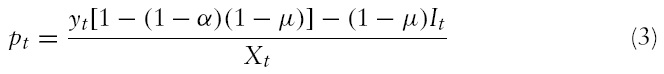
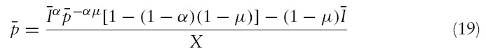
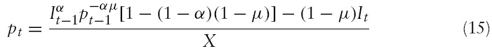
Equation (3), obtained using equation (2), expresses the domestic real exchange rate as a function increasing in domestic output and investment but decreasing in exports.
Inequality (4) specifies that the ability of domestic entrepreneurs to invest is limited by their wealth such that entrepreneurs can borrow at most (1 +
Equation (5) shows that the return of domestic bonds is equal to the marginal productivity of capital. Because a share

5 One unit of domestic good saved in

units of capital before the production takes place and therefore the return on domestic bonds should (by arbitrage) be equal to

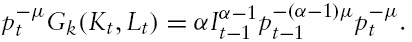
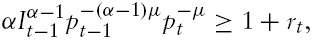
According to equation (6), entrepreneurs will not borrow beyond the point at which the real return on domestic investment, determined by equation (5), equals that on foreign bonds. It is similar to uncovered interest rates parity (UIP), which compares the rate of return of foreign bonds

and the return (converted into foreign goods at
Equation (7) imposes that investment cannot be negative. Equation (8) defines the net wealth of entrepreneurs as the difference between the share of domestic revenue attributed to the owners of domestic capital and the actual value of the debt that they owe to lenders.
We introduce two equations that represent the logic extension of Krugman’s model and are important to our understanding of the dynamic features of a crisis-prone economy:

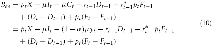
Equation (9) describes the evolution of foreign debt used by domestic entrepreneurs to finance an investment greater than their wealth. It represents their balance-sheet constraint.
Equation (10) represents the external equilibrium condition or balance of payments. Under a flexible exchange rate regime (i.e.,
Assume that entrepreneurs are risk neutral and maximize their firms’ profits in period

i.e. the marginal rate of return of capital is higher than the cost of financing investment, entrepreneurs will borrow from abroad the maximal amount allowed by the leverage constraint (4), which is therefore binding. Otherwise, equation (4) will not be binding.
At the equilibrium in the international financial market, the absence of arbitrage opportunity between domestic and foreign currency denominated bonds implies that equation (6) is verified with equality:

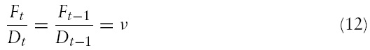
The ratio of foreign currency (or goods) denominated debt relative to domestic currency denominated debt is assumed for simplicity to be constant and equal to

The ratio
Foreign banks would pay attention to the wealth left to entrepreneurs after the payment of principal and interests. Using equation (1) with

equations (8) and (11)–(12), we obtain:

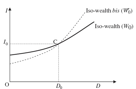
If
For a given wealth

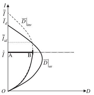
An iso-wealth curve represents the combinations of foreign debt and investment that ensure a constant wealth (Figure 1). A given combination of investment and foreign debt (

7
The model has nine endogenous variables and is solved in two steps. The first step of the resolution consists of solving the difference equations for
Under the assumption that the risk-neutral entrepreneurs, when their wealth is low enough, use the leverage financing so that equation (4) is binding, i.e.

The dynamics of

Difference equations (15)–(17) describe the dynamic behavior of real exchange rate, investment and foreign debt. They are non-linear and cannot be solved explicitly. The static and dynamic properties of the system can be studied with the help of a phase diagram.
4Here, we introduce this assumption to close the small open-economy model in order to avoid these entrepreneurs accumulating an infinite amount of wealth. This assumption might not be plausible for describing some emerging economies having sufficiently accumulated capital. As illustrated by recent international developments of South Korean firms, ambitious entrepreneurs might be tempted to invest in international financial assets and/or industrial projects. See Schmitt-Grohé and Uribe (2003) for other ways of closing the model. 5Aproportion, 1 − μ, of the investment goods is built with domestic goods and another proportion, μ, with foreign goods, the price of one unit of investment goods in period t − 1 measured in terms of domestic goods is Hence, one unit of domestic goods is equal to units of last period’s investment goods. 6This assumption partially reflects the original sin hypothesis advanced by Eichengreen and Hausmann (1999) who define it as a situation in which the domestic currency cannot be used to borrow abroad or to borrow long term, even domestically, and which was modified by Eichengreen et al. (2005) who discard the domestic element of original sin and redefine original sin as a situation in which most countries cannot borrow abroad in their own currency. 7According to equation (14), this is the case when there is: (i) an increase in that reduces entrepreneurs’ wealth; (ii) a decrease in X, since this implies according to equation (3) a real depreciation, decreasing the current value of domestic product but increasing the value of foreign debt measured in domestic currency; (iii) an increase in μ that, by increasing the demand for foreign goods, implies a real depreciation and hence has a similar effect as a decrease in X. However, an increase in α has ambiguous effects on the wealth. It induces an increase in the revenue attributed to capitalists as well as a real depreciation (owing to the higher productivity of existing capital and hence higher output, and a higher part of the revenue that is exported) with the above-mentioned effects. Finally, a variation of λ has no effect on the iso-wealth curve.
The steady state equilibrium, where variables are denoted by an upper bar, is attained when the dynamic effects of shocks are fully realized. Since optimal investment verifies

the steady state investment must satisfy:

Given

the highest steady state investment,

equalizes the marginal productivity of capital and the opportunity cost of investing.
The steady state counterparts of equations (15)–(17) are given as follows:


The steady state equilibrium of the reduced dynamic system is defined by the vector

Given

equation (19) determines

Equation (20) corresponds to the combination of investment and foreign debt along the quickest wealth-accumulation path limited by condition (18). Given the real exchange rate, it would determine a ‘financeable’ level of investment that would occur if equation (4) was binding and the maximal credit (or debt capacity) that could be granted to domestic firms. Equation (21) is the solvency constraint of entrepreneurs,which implies that the surplus ofwealth over investment is equal to interest payments on foreign debt. Since the foreign debt is uniquely contracted by entrepreneurs, their solvency constraint is also the economy’s external solvency constraint. Thus, equation (21) is equivalent to the steady state counterpart of equation (10) meaning that, in the long-run, the trade surplus must be equal to interest payments on foreign debt.
Substituting

into equations (20) and (21) and rearranging the terms lead to

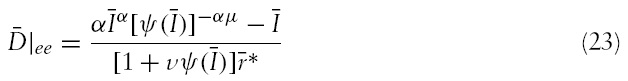
where

and

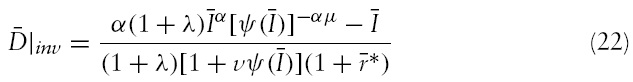
denote, for all levels of investment, the highest steady state debt compatible with the leverage constraint and the external solvency constraint respectively. Equations (22) and (23) constitute a sub-system incorporating the effects of the real exchange rate on wealth, i.e. balance sheets, and can be solved to obtain

and

taking account of equation (18).
The curves

and

could be represented as in Figure 2, where

represents the intersection point of these two curves, and

and

respectively the higher intersection point of

and

with the axis

with

Using equations (18) and

the set of feasible combinations of debt and investment is constituted of AB
and OB

For

risk-neutral entrepreneurs will fully use their debt capacity allowed by equation (4) corresponding to the most rapid wealth growth. When

is attained, entrepreneurs will reduce the leverage to a level smaller than (1 +
The relative position of

and

depends on the value of

it does not affect

These two curves rotate counter-clockwise around

but has no effect on the external solvency constraint. Finally, an increase in
The foreign debt is assumed to be non-negative, i.e.

translating the assumption that, after having exhausted domestic investment opportunities, entrepreneurs will consume the surplus of their revenue over investment. Therefore, there are only two steady-state equilibria, i.e. the point A where foreign debt is zero and investment equals

and the point

the intersection point of

and

is not a steady state equilibrium.
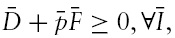
4. Dynamics and Mechanism of Financial Crisis
Since the difference equations (15)–(17) are non-linear, it is not possible to deduce algebraically the sign of Δ
To the right (left) of

because the external debt is too high (low) in the sense that the trade surplus is not sufficient to pay interests on the existing foreign debt and the latter keeps increasing due to the current account deficit, Δ

the foreign debt is smaller than the debt capacity of entrepreneurs. Thus, the latter can invest more and more to increase their wealth, implying that Δ

the foreign debt is too high to satisfy the leverage constraint and the wealth will be insufficient to sustain the past level of investment. Thus, investment must be reduced, implying down arrows for areas 2–7.
The equilibrium A is stable since any trajectory originated in its near neighborhood converges to it. The equilibrium O is unstable because a small wealth is sufficient to start a wealth accumulation process with more and more investment and foreign debt, finally leading the economy to the equilibrium A.
As in Krugman (1999), the foreign debt capacity of entrepreneurs depends on their wealth, which in its turn depends on the amount of such debt because the volume of capital inflows affects the terms of trade and hence the valuation of foreign-currency denominated debt. Therefore, a decline in capital inflows can adversely affect the balance sheets of domestic entrepreneurs, reducing their ability to borrow and hence further reducing capital inflows.9
In area 1, given the high rate of return on investment, the wealth accumulation is delayed by not fully using the debt capacity. In contrast, area 7 is characterized by over-investment so that entrepreneurs reduce investment and foreign debt. In both areas, the foreign debt is smaller than the debt capacity determined by the leverage constraint (4) and is compatible with the external solvency constraint. Hence, in these areas, the probability of a crisis is zero and there will be nothing that resembles an Asian-style financial crisis.
In area 6, despite over-investment, there is no financial risk in the short run because the foreign debt is lower than the debt capacity determined by the leverage constraint. However, entrepreneurs must reduce investment to

and the foreign debt correspondingly to avoid that the foreign debt, which exceeds the level compatible with the external solvency constraint, continues to increase to attain an unsustainable level in the long term.
However, on the curve OB and to the left of this curve (areas 2–5), the risk of financial crisis depends positively on the level of debt and negatively on the level of net wealth.
In areas 2 and 5, the foreign debt is greater than the debt capacity determined by the leverage constraint but is compatible with the external solvency constraint. If the economy is found in the area 2 after a negative shock, the realized temporary equilibrium after adjustment of the international lending can be more or less favorable, depending on the confidence of international lenders placed on these entrepreneurs and on the perspectives of the domestic economy. For example, given an initial wealth

In areas 3 and 4, both leverage and external solvency constraints are violated. This implies that the risk of financial crisis is very large. Compared with area 3, area 4 is characterized by higher net wealth and overinvestment. If a financial crisis occurs, it will be less violent in area 4 than in area 3, where the level of foreign debt is too high given the net wealth of entrepreneurs. In area 3, except when the foreign debt becomes too large, lenders could recover all or most of their lending. If they wait, the situation could deteriorate so that they make a loss while most entrepreneurs are bankrupted. In area 4, international lenders could react negatively to over-investment, except when the foreign debt is quite low compared with the net wealth of entrepreneurs.
A prosperous economy pursuing a quick wealth-accumulation path, such as OB, can be suddenly hit by a capital outflow due to spill-over effects (Masson, 1999), i.e. a crisis in one country may affect other emerging markets by contagion due to linkages operating through trade, economic activities or competitiveness.A typical example is a currency devaluation of a rival country in crisis,which reduces domestic exports. In such an event, an economy initially on the path OB could be found to the right of

or in the worst case to the right of

as these curves rotate counter-clockwise following a fall in exports. This could make the initial temporary equilibrium with high investment and high foreign debt unsustainable judging by the leverage constraint and/or the external equilibrium condition. If the leverage constraint is violated while the external solvency constraint is respected, the panic of lenders and the resulting financial crisis might not be too severe since the reduction of liquidity in the domestic economy will not bankrupt most entrepreneurs. In effect, a reduction in exports will negatively impact the entrepreneurs’ wealth (the iso-wealth curve rotates counter-clockwise) since it implies a real depreciation and hence an increase in the value of foreign-currency debt measured in domestic currency. If both constraints are violated, the panic of lenders and the resulting financial crisiswould be severe.To analyze the severity of a crisis, one must appropriately consider factors such as initial wealth, leverage multiplier, amplitude of the fall in exports and other structural parameters of the economy. For emerging market economies that initially offer a high rate of return of capital, the crisis could result from earlier choices of entrepreneurs who underestimate the effects of adverse shocks on the financial stability and their repercussion on the rate of return of the capital.
Any temporary equilibrium along the curve OB is submitted to the risk that a loss of lenders’ confidence could be validated by a financial collapse if these lenders radically change their attitude and behavior towards domestic ntrepreneurs. In normal times, domestic entrepreneurs could finance their investment by fully using the debt capacity determined by the leverage constraint. But in bad times (e.g., a financial crisis hits other emerging market economies), as the debt is short-run, panicking international lenders could arbitrarily reduce the leverage multiplier to a level that guarantees the repayment of principal and interests, translating an increase in their risk aversion or a loss of their confidence on future perspectives of the domestic or/andworld economy.This induces the curve

to rotate counter-clockwise while the curves

and iso-wealth remain unaffected. A reduction in the leverage multiplier might not be sufficient to lead a financial crisis to occur, except when the pessimistic expectations of lenders are realized. If wealth is not affected, investment and foreign debt will adjust orderly towards lower levels.
Under a flexible exchange rate regime, a severe and instantaneous reduction of investment and foreign debt can take place when some shocks modify hugely and adversely the current and future real exchange rates. Lenders would examine attentively to what extent any important shock of this kind will reduce entrepreneurs’ wealth and hence increase the risk of economic and financial collapse leading to a low level of investment and wealth. This scenario is more probable when investment and foreign debt are both jumping variables. If investment is only partially amortized in every period and the foreign debt is long term, the immediate collapse will be less severe. However, the financial crisis, while less violent than the one with sudden withdrawal of foreign lending, could be long-lasting if appropriate policy measures are not taken by national authorities and/or international financial institutions.
Even though the basic part of this model is the same as in Krugman, the crisis mechanism here is somewhat different. In fact, Krugman worked with three equilibria that are made possible by using a static analysis. A financial crisis then corresponds to a jump from the equilibrium with high investment to the one with zero investment since all entrepreneurs are bankrupt, given that the intermediate equilibrium is unstable. Examining the dynamic model, we have shown that that there are only two steady state equilibria. A financial crisis is then a dynamic phenomenon of an emerging market economy that uses extensively foreign currency denominated debt to finance its development. It is a jump, susceptible to occur when some factors make international lenders panic, from one dynamically unstable trajectory of wealth-accumulation with high foreign debt and high investment to another trajectory with less investment and lower foreign debt. When a severe financial crisis occurs, not all entrepreneurs are systematically bankrupt. The economic and financial collapse does not imply that the previous investments were unsound. The problem is, instead, one of financial fragility in a dynamic context.
We have previously analyzed the mechanism of financial crisis using the example of a crisis by contagion. Our dynamic setting can be easily used to analyze the impacts of factors leading to the financial fragility. Generally, these factors could also induce a financial crisis if they come to change adversely. They matter because they make the circular loop from past investment to real exchange rate to balance sheets to current investment more powerful. But they didn’t explain why the Asian financial crisis occurred. All afflicted Asian economies were peculiarly vulnerable to a financial crisis owing to a high leverage and unusually high levels of foreign currency debt. These borrowings have placed them before an increased risk of financial collapse if the real exchange rate depreciates. We discuss in the following some of these factors, i.e. high leverage, large foreign-currency debt relative to exports, and monetary policy shocks in industrial countries.
High leverage increases the speed of wealth accumulation by domestic entrepreneurs but also accelerates thewealth destructionwhen the economy is hit by adverse shocks. It makes the economy more vulnerable to a negative change in lender’s attitudes towards domestic entrepreneurs. An increase in leverage, i.e. a higher

to rotate clockwise without modifying the position of

Whatever is the value of

is always to the left of


The new quickest wealth-accumulation path will be nearer to the external solvency constraint. This increases the fragility of the economy by increasing the probability that the economy violates both leverage and external solvency constraints in the event of negative shocks inducing these constraints to rotate counterclockwise.
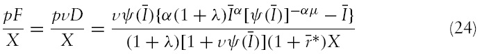
The ratio of foreign-currency debt relative to exports is a complex indicator that is not clearly discussed by Krugman. A large ratio of foreign-currency debt relative to exports can be due to multiple factors. Using equations (12) and (22), the ratio can be written as:

An increase in

and

while an increase in

will make these firms more vulnerable to a financial crisis because, in the event of such a crisis, the outflows of capitalmust be financed by the surplus of the trade balance. The ratio

also depends on investment and hence the stage of economic development. It should be noticed that some parameters or exogenous variables, such as

and
The monsoonal effects could be one possible explanation of the 1997 Asian crisis. The monsoonal effects emanate from the global environment (in particular, from policies in industrial countries), and sweep over all emerging countries to a greater or lesser extent (Masson, 1999). Thus, a monetary contraction in a worldleading country could considerably raise the financial costs of investment for an indefinite horizon and hence put some emerging market economies under great financial pressures. One important factor, which was present before the Asian financial crisis, is the high 3-month Libor interest rate (Kwack 2000). In effect, previous to the crisis, the Fed has adopted a restrictive stance for its monetary policy, inducing the interest rate to rise on international financial markets. According to equations (18), (22) and (23), an increase in

and

and hence the curve OB to rotate counterclockwise. An increase in the foreign interest rate reduces the foreign funds that domestic entrepreneurs can borrow because it diminishes their wealth and hence their debt capacity. If wealth is high enough at the initial temporary equilibrium, the resulting adjustment can place the economy on the new wealth-accumulation path. Ifwealth is low, the foreign debt can instantly jump to a lowlevel if it is short term and hence induces a violent financial crisis. Increasing the part of long-term debt reduces the severity of the crisis but can make the latter long-lasting.
8Using equation (16), we have This is not a complete derivation since according to equation (15) pt is a function of It and It−1. For and without taking account of the constraint when Dt−1 is higher than we have ΔIt < 0 and vice versa. In the space delimitated by and the axis I, and above the lineAB, the lack of profitability leads rational entrepreneurs to reduce investment. Using equation (17) to obtain we have ΔDt > 0 and vice versa. 9It is largely documented that the Asian countries affected by the 1997 financial crisis had a balance of payments characterized by large current account deficits compensated by net inflows of foreign capital.
The dynamic setting can be easily used to re-examine three policy issues considered by Krugman (1999), i.e. preventive measures against financial crisis, policy during the financial crisis and rebuilding the economy after the financial crisis. It should be noticed that the present framework, formulated in nonmonetary terms, is more adapted for analyzing the situation of emerging market economies exposed to foreign currency debt under a floating exchange rate regime.10 However, an exchange rate peg can be mimicked by a real exchange rate peg. Henceforward, we do not explicitly consider the exchange rate peg in the following.
Regarding the preventive measures against financial crisis, Krugman has argued that the imposition of Chilean-type restrictions on short-termborrowing denominated in foreign currencies, which reduces the short-term foreign-currency exposure, could not allow emerging market countries to significantly reduce the risks of being forced into a crisis by a loss of confidence. In addition, as long as a country has free convertibility of capital, short-termforeign loans are only one of many different possible sources of capital flight. Our dynamic analysis allows a more nuanced analysis since we can consider the case where only a small part of foreign loans is short term, foreign debt will not be a totally free jumping variable and will not fall to zero whenever there is a financial crisis.
Consider again the example of a contagious financial crisis in a competing country, which decreases the expected exports of the domestic country in the future. As analyzed in Section 4, such an event reduces the sustainable level of foreign loans by reducing the entrepreneurs’ net wealth, leading all three curves


and iso-wealth to rotate counterclockwise. Therefore, a temporary equilibrium on the quickest wealth-accumulation path before the financial crisis is not sustainable anymore. Denote by

the new location to which the curve

rotates counterclockwise. A high level of long-termforeign debt implies that the financial crisis could be less violent but long-lasting.The refusal of the holders of short-term foreign debt to roll it over could generate an exchange rate depreciation that deteriorates the balance sheets and bankrupts some entrepreneurs until the foreign debt is sufficiently low
Nonetheless, a higher rate of return of capital allows entrepreneurs, having survived the crisis, to regain the confidence of international lenders.
The nuances thatwe introduce in the analysis of the impact of the financial crisis does not put into question Krugman’s proposition about the appropriate prophylactic policy, i.e., to avoid any transmission of international crisis to the domestic economy, it is necessary to discourage firms from taking on foreign-currencydenominated debt of any maturity. In effect, the real-exchange-rate impact of adverse shocks has negative effects on domestic investment financed with such debt but lets an economy without it be unaffected. These effects are magnified through balance-sheet effects to cause economic distress if such debt is high.
The dynamic setting can be used to analyze the policies adopted during the Asian financial crisis. In the period before 1997, Asian countries have grown rapidly and liberalized their capital account as urged by the IMF while operating a nominal exchange rate peg. The peg of Asian monies to the US dollar is an important characteristic of these countries. Avoiding the risks of financial trauma due to the foreign currency debt was a major reason why the IMF advised its Asian client countries to follow the much-criticized ‘IMF strategy’, which consists of defending their currencies with high interest rates rather than simply letting them devaluate.11 We can get some insight into the nature and consequences of the IMF strategy by imagining that the effect of that strategy is to hold the real exchange rate
The phase diagram (Figure 3) can be modified to examine such a type of policy in the casewhere the domestic economy is submitted to a contagious crisis.13 Even though the contagion due to the crisis in neighboring countries leads international lenders to think that the foreign debt is too high for the leverage constraint to be respected, the above measure is justified if the level of investment before the crisis is less than

and if the foreign debt is always compatible with the external solvency constraint. The anticipated depreciation of domestic currency (and hence that of the real exchange rate) indicates a possible temporary equilibrium with smaller wealth and lower investment following a counterclockwise rotation of the curve’s iso-wealth and

Hence, maintaining the temporary equilibrium at the point C can consume a lot of financial resources given that some foreign lenders will reduce their lending. To maintain the level of investment corresponding to point C, the IMF’s financial aid must be enough to compensate for the credit lost by firms so as to allow investment to continue. If the IMF funds are used to defend the nominal exchange rate peg, the aid must be large enough to substitute all private foreign lending capital,which could quit the country at the official nominal exchange rate. Such a measure could be successful if shocks are temporary.
Considering the bad equilibrium with zero investment, Krugman (1999) suggested that the main problem with the post-crisis rebuilding of the economy was that the entrepreneurs who drove investment and growth before the crisis are now effectively bankrupt and unable to raise capital. Our nuanced results about the severity of financial crisis following a foreign exchange crisis, suggest that the post-crisis rebuilding of the economy could be looked at with more optimism in the sense that, generally, the economy hit by a financial crisis can return to rapid growth without waiting for foreign aid and a new set of entrepreneurs.
In the dynamic setting, the situation depends on the initial levels of wealth and foreign currency debt of every individual entrepreneur. If the aggregate wealth of entrepreneurs after the devaluation of the domestic currency is high and only slightly affected by the twin crises, many entrepreneurs can survive. They are able to reimburse their foreign debt and continue to develop in a context with less competition and higher profitability since the investment level is lower. This, then, will create a new wave of development soon after the twin crises. In this case, the efforts focused on bank restructuring and recapitalization are sufficient.
However, these efforts will not be sufficient in the case where the aggregate wealth after the devaluation is near zero or negative and most entrepreneurs have been bankrupted. Even if a big wave of development can be initiated by non-bankrupted entrepreneurs once the dust of the crises has settled, the deep economic recession is too costly in the short run. Solutions proposed by Krugman, such as rescuing bankrupt entrepreneurs through some kind of ‘private sector Brady Plan’, and/or growing a new set of entrepreneurs and/or welcoming foreign direct investment, are needed to reduce the negative economic and social consequences of the twin crises and to accelerate the economic recovery.
10This is, to some extent, the case in most Central and Eastern European countries and Iceland. 11One mistake of Thailand’s government was to raise the local interest rate, since the interest rate parity theorem tells us that those speculators who have already sold short baht in the forward market will be enriched, not hurt. Moreover, this can hurt entrepreneurs and hence precipitate a financial crisis (Miller, 1998). 12A controversial measure used by Malaysia during the 1997 crisis – imposing a strict curfew on capital flight, and which is not discussed here in order to limit the length of the article – could also rule out the possibility of a downward financial spiral by maintaining the real exchange rate constant. In Figure 3, it consists of maintaining the economy at the point C by keeping unchanged the real exchange rate and by not letting the foreign lenders reduce their lending. It is justified by the fact that standstill agreements on foreign-currency debt are not sufficient to avoid the crisis. It is efficient only if the adverse shocks are temporary and over-investment not observed. 13For detailed analysis about how the curves shift, see Section 4.
This article analyzes the dynamic implication of the Krugman’s (1999) model by extending it to explicitly take account of wealth accumulation and external equilibrium constraints. Our dynamic analysis complements his discussion of factors susceptible to induce financial fragility and crisis while suggesting some nuanced crisis scenarios and policy implications.
This study has shown the existence of two equilibria. The equilibrium characterized by zero investment and zero foreign debt is unstable since a small amount of capital could put the economy on a wealth-accumulation path leading to the other equilibrium with positive investment and zero debt. In this dynamic process, an economy largely exposed to foreign-currency denominated debt can be hit by a financial crisis analyzed as a jump from one wealth-accumulation path to another one with lower investment and lower foreign debt. The violence of such a crisis will depend on the part of short-run debt in the total foreign debt. In contrast, Krugman obtained three equilibria through a static analysis. Thus, a financial crisis is considered as a jump from the equilibrium with high investment and high debt to the stable one where all entrepreneurs are bankrupt and do not invest.
Furthermore, the dynamic analysis allows discriminating the severity of financial crises and their economic consequences according to the pre-crisis wealth. It allows gaining more intuition about the adjustments induced by different anticrisis policy measures. In particular, our analysis suggests that even during a severe financial crisis, not all entrepreneurs are bankrupt. Since those having survived the crisis could jump-start a wealth-accumulation process, policy measures other than bank restructuring and recapitalization are not always needed to rebuild the economy, except when the consequences of such a crisis are very severe.