The global economy has recently experienced exceptional levels of volatility. Despite the fact that such volatility was mostly apparent in financial markets, international productionwas also harshly hit.The decline in global output during the most recent downturn is comparable to that during the Great Depression. Individual countries experienced large-scale contractions during the latest recession. For instance, in Germany, real gross domestic product (GDP) per capita, which grew 2% on average since 1960 (with a standard deviation of 2.3%), contracted by 6.7% in 2009.
The volatility of output growth is a potentially important determinant of economic growth, as output volatility raises economic uncertainty, hampering investment due to its irreversible nature, which in turn leads to lower long-term economic growth (Bernanke, 1983).
Despite the fact that studies investigated the relation between output volatility and growth (see, for instance, Ramey & Ramey, 1995; Lee, 2010), little is known about output growth volatility spillovers among countries. In addition, the empirical literature on output growth dynamics during the latest recession is limited. Antonakakis and Scharler (2011) examined output growth dynamics during US recessions and found that the 2007 to 2009 recession was associated with unusually highly synchronized output growth dynamics in the G7 countries. The source of such high synchronization may be attributed to financial integration and contagion (Mendoza&Quadrini, 2009). As a result of the high level of integration of the economies, shocks experienced by one country have increasingly important implications for other countries.
The motivation for this study is to investigate the interdependencies of GDP growth rates and their volatilities across the G7 countries under a multivariate GARCH framework. Put differently, the interaction of GDP growth of one country with the others is examined. More importantly, we investigate GDP growth volatility spillovers across countries by examining how own-country shocks and volatilities as well as cross-country shocks and volatility co-movements impact on GDP growth volatility of one country and how they are transmitted across countries.
In particular, the contribution of this paper is twofold. First, we obtain timevarying measures of variances and covariances by the use of the BEKK-MGARCH model proposed by Engle and Kroner (1995).1 Even though this model has been applied solely to financial data so far, we argue that this approach is a strong candidate for the subject of the present paper, yielding more elaborated measures than rolling-time windows to construct time-varying measures of variances and co-variances. Second, we extend the sample period up to the fourth quarter of 2010, which allows us to exploit the potentially valuable source of variation in the data due to the recent financial and economic crisis.
The remainder of this paper is organized as follows. Section 2 describes the methodology employed and data used. Section 3 presents and discusses the estimated results. Section 4 summarizes the results and concludes.
1The acronym BEKK stems from the joint work of Baba, Engle, Kraft and Kroner.
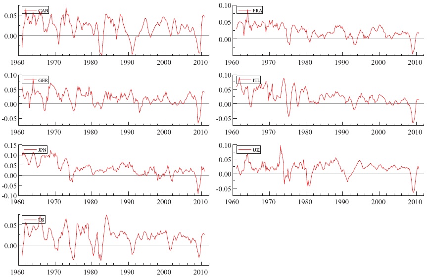
The dataset consists of quarterly observations of real GDP per capita in the G7 countries over the period 1960Q1 - 2010Q4 obtained fromOECDMain Economic Indicators database.We calculate output growth as the fourth quarter difference of the log of quarterly realGDPper capita, yielding stationary series of annualized output growth in the G7 countries.2 These series are plotted in Figure 1 where it can be seen that, in general, the largest decline of GDP was recorded in the most recent downturn. Table 1 presents the descriptive statistics of these series. Generally, annual GDP growth rate in the G7 countries during the sample is 2% with Japan the only exception with an annual GDP growth rate of 3%. Yet Japan is subject to higher shocks as it experiences the largest deviations in output growth (3.6%) compared with the remaining G7 countries (where standard deviation is around 2%).
According to the pairwise unconditional correlations in Table 1, GDP growth of all G7 countries is positively interrelated. The highest correlations are between countries that are in close geographical proximity such as Canada and the US (0.7702), and France and Italy (0.7767),whereas, the lowest correlation is between Japan and Canada (0.3541). An additional feature of the data, which will be addressed in the econometric analysis, is the presence of ARCH effects in the residual series of a VAR model for GDP growth.
[Table 1.] Descriptive statistics of GDP growth in G7 countries
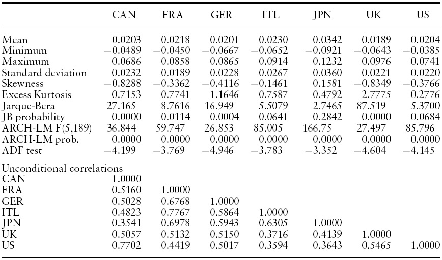
Descriptive statistics of GDP growth in G7 countries
To address the transmission of GDP growth and GDP growth volatility among the G7 countries we employ the BEKK-MGARCH model originally proposed by Engle and Kroner (1995). This is a novel contribution of the present study as, to the best of our knowledge, this model has not been applied to investigate output growth volatility transmission.
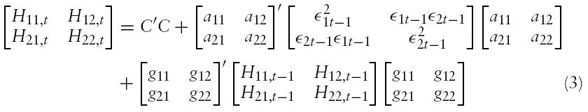
The following conditional expected GDP growth equation relates each country’s GDP growth to its own and other countries’ GDP growth, lagged

where
There exist various parameterizations of the conditional variance–covariance matrix,

where

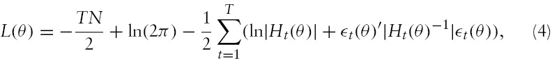
Under the assumption of normally distributed random errors, the loglikelihood function for the BEKK-MGARCH model is given by:

where

parameters in the conditional variance and
2According to the Augmented Dickey-Fuller (ADF) test results in Table 1, the null hypothesis of a unit root is rejected at the 0.01 level of significance in all cases. 3Positive semi-definiteness of the conditional variance-covariance matrix is ensured by construction, which is a necessary condition for the variances to be positive.
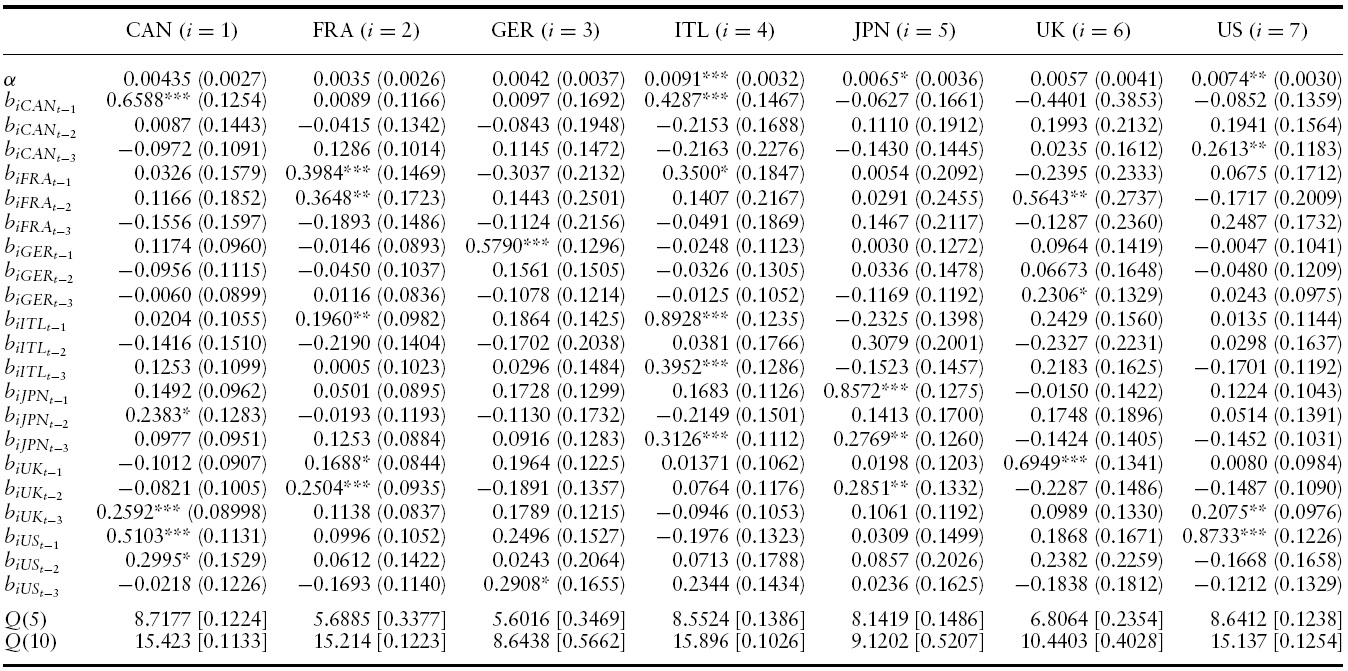
The estimated conditional mean and variance equations with the associated robust standard errors, likelihood function values and misspecification tests for the G7 countries’ output growth are presented in Tables 2 and 3 for the full sample period.4 Specifically, a VAR(3)-BEKK-GARCH(1,1) turned out to be the preferred specification in terms of standard residual diagnostics (serial correlation and overfitting tests) and the AIC and SBC criterion.

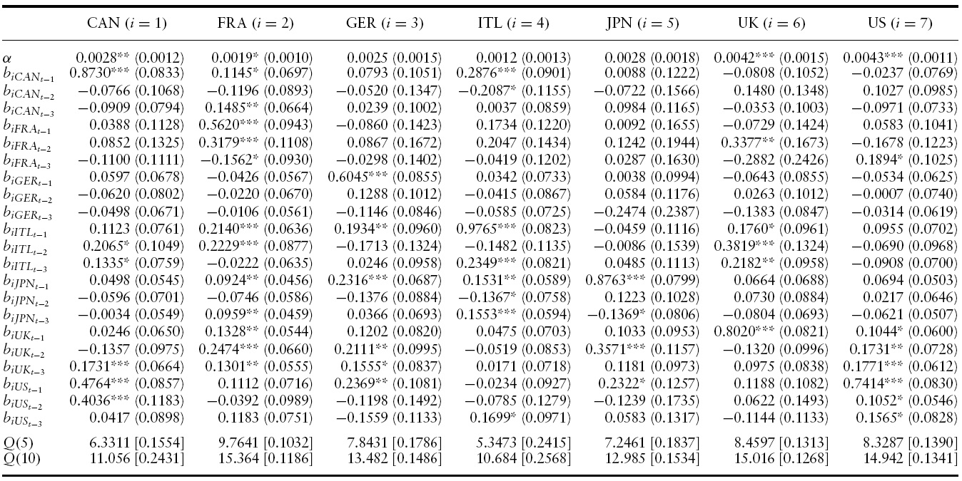
Conditional Mean Results of VAR(3)-BEKK-GARCH(1,1) model for GDP growth in the G7: 1960Q1?2010Q4
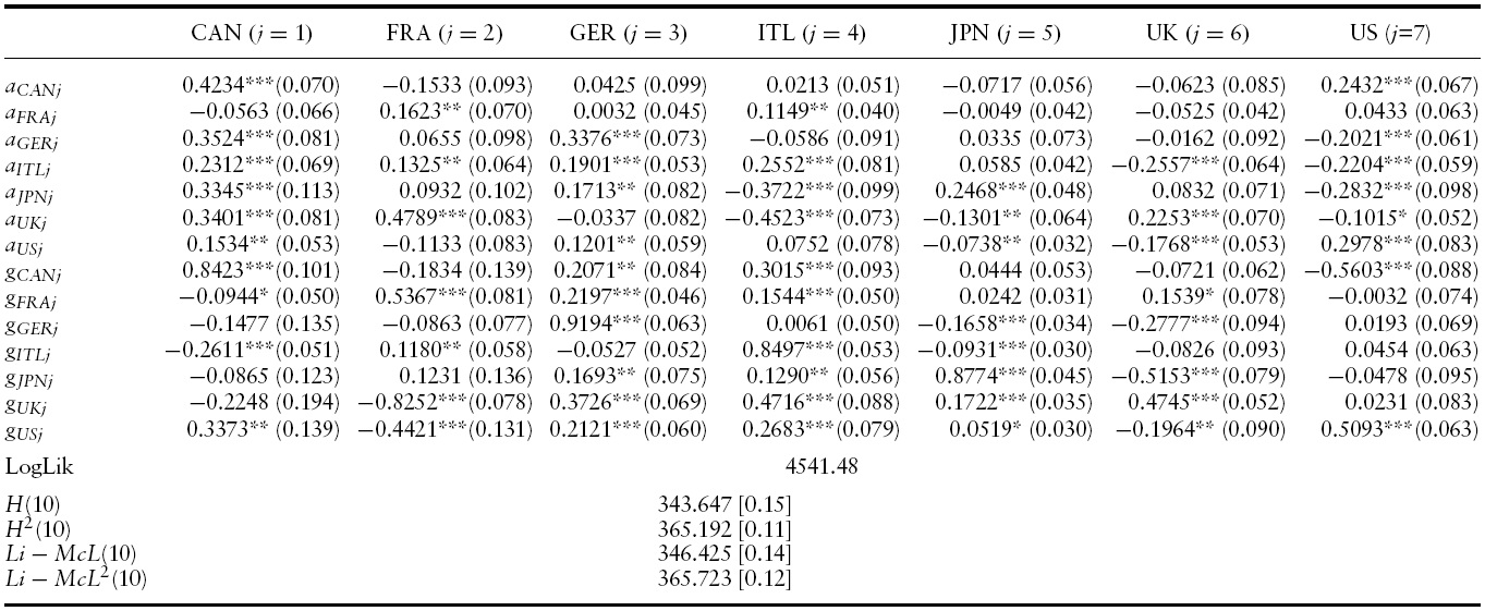
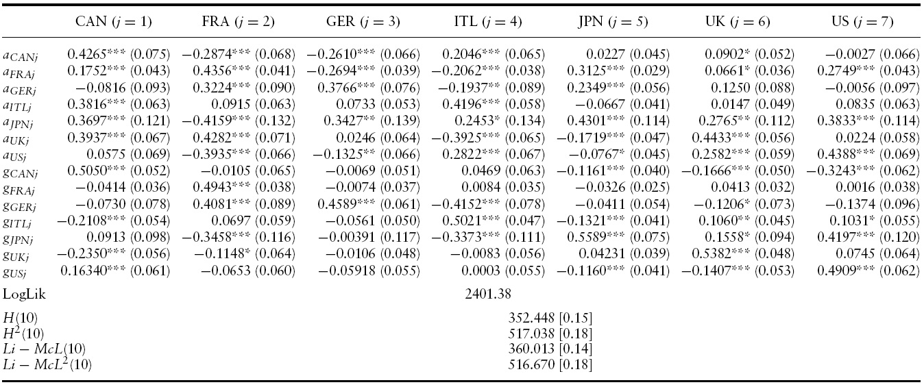
Conditional variance results of VAR(3)-BEKK-GARCH(1,1) model for GDP growth in the G7: 1960Q1?2010Q4
According to the conditional mean of output growth of the VAR(3)-BEKKGARCH(1,1) model reported in Table 2, all countries exhibit significantly positive and high own mean spillovers from at least their own first lag of output growth. The parameter estimate for the own mean spillover ranges from 0.5325 in France to 0.8950 in Japan indicating a high degree of persistence.
Importantly, there are significant lagged mean spillovers from many of the G7 countries to many of the remaining others. Among all (147) lagged estimated coefficients,32%(47) of them are significantly positive and2%(3) are significantly negative, indicating a high degree of business cycle synchronization in the G7 countries throughout our sample.5
For instance, in the case of Canada, the effect of previous quarters annualized growth rate of US (first and second quarter), Italy (second and third quarter) and UK (third quarter) will Granger-cause an increase on the current quarter annualized growth rate of Canada. Put differently, previous output growth changes in the US, Italy and the UK tend to synchronize their business cycles with that of Canada in the current period.
In United States, only previous third and first–third quarter annualized growth rates of France and the UK, respectively, have a positive direct impact on current quarter annualized growth rate in the United States (apart from its own lags).
Overall, these results suggest that, on average, short-run output growth changes in many of the G7 countries are associated with significant output growth changes in many of the remaining countries, indicating the presence of a high degree of business cycle synchronization with quarter annualized growth rate lags. This is in line with the literature 9see, for instance, Stock & Watson, 2005) and can be attributed to the increased integration of goods and financial markets (Mendoza & Quadrini, 2009).
3.2 Output Growth Volatility Spillovers
Having evaluated the dynamics of output growth spillovers we now present the results of the conditional variance of the VAR(3)-BEKK-GARCH(1,1) model for output growth volatility spillovers across the G7 countries.
The conditional variance–covariance equations of the VAR(3)-BEKKGARCH(1,1) model effectively capture the own-volatility and cross-volatility interdependencies of output growth among the G7 countries. Table 3 presents the parameter estimates for the conditional variance–covariance matrix,
Own-innovations spillovers in all G7 countries are significant, indicating the presence ofARCHeffects.The own-innovation effects range from0.1623 in France to 0.4234 in Canada. That is, past output growth shocks in Canada will have the strongest impact on its own current volatility compared with country-specific output growth shocks in the other six countries.
Turning to cross-innovation effects of GDP growth in the G7 countries, past innovations in most countries exert an influence on GDP growth volatility of the remaining countries. Nevertheless, cross-volatility shocks are generally lower than the own-volatility shocks. This means that past cross-volatility shocks have aweaker effect on current conditional volatility in a country than country specific volatility shocks of that particular country.
In the GARCH set of parameters one can observe that own-country and cross-country volatility spillovers vary in magnitude and sign, respectively, across countries. Own-country volatility spillovers range from0.4745 in theUKto 0.9194 in Germany. This suggests that own-past output growth volatility spillovers in the UKhave theweakest effect on its own-current conditional output growth volatility, compared with own-volatility spillovers in the remaining countries.6
In addition, second-moment interdependency can be detected as the conditional variance in each market is also affected by persistence in the other countries. Moreover, the negative coefficients of the off-diagonal elements of the conditional variance matrix indicate possible asymmetries in interdependencies.
It should be noted that the off-diagonal elements of
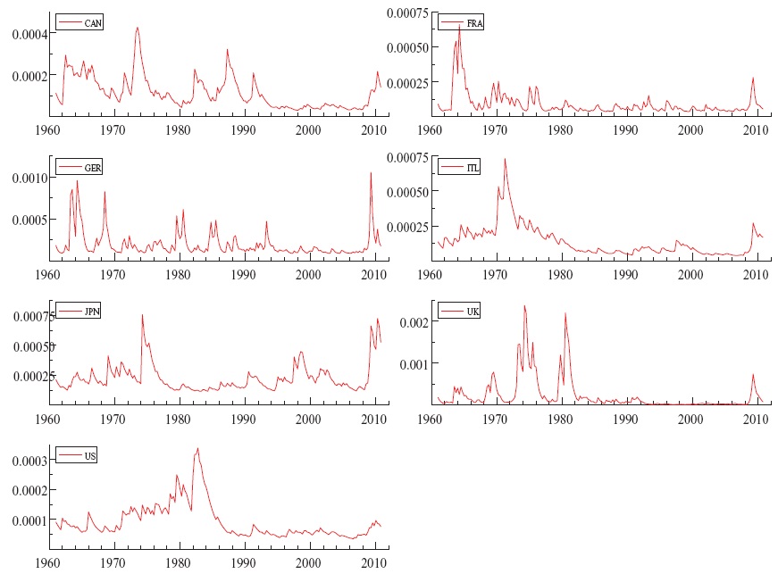
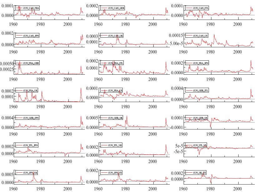
Figures 2 and 3 plot the conditional variances and covariances of the BEKK model and reveal some important features. First, in line with the empirical literature (see, for instance, Stock & Watson, 2005), international volatility and business cycles synchronization declined since the mid-1980s, a period known as the great moderation. Nevertheless, international volatility and business cycles co-movements generally reached a peak during the most recent worldwide crisis (Antonakakis & Scharler, 2011). These results suggest a probable end to the great moderation and a beginning of a new era of increased business cycle comovements and spillovers. Put differently, the global economy seems to have passed from the period of the great moderation to the period of the great integration.
Before we proceed with the impulse response analysis it is imperative to check whether our estimation results are biased due to misspecification. Since our sample consists of periods of high volatility (during the 1970s and the 2008–2009 recession) and periods of lower volatility (since the mid-1980s and before the latest recession), there might be structural breaks present in the conditional mean and/or volatility process that could bias our estimation results reported in the previous section.
Therefore, we perform the structural break test proposed by Inclan & Tiao (1994) to detect such breaks. The test is based on the iterative cumulative sums of squares (ICSS) algorithm.
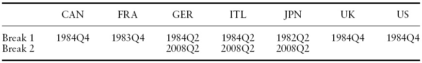
The results of this test, which are given in Table 4, indicate a break in the unconditional variance at 1984Q4, which coincides with the date when the world economy entered the great moderation. Therefore, we split our sample in two subperiods: the pre-1985 and the post-1985 period.7
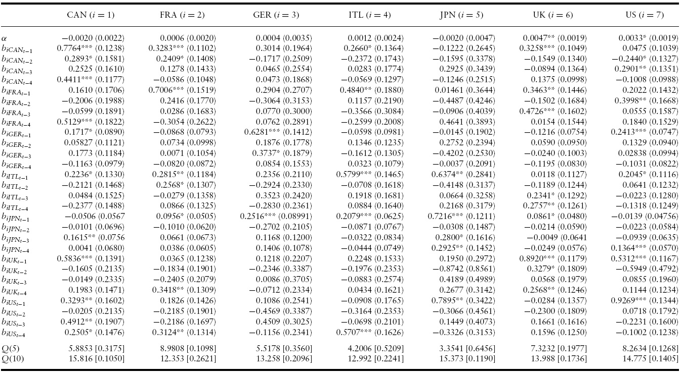
After a battery of tests, the most appropriate specifications to fit our data for the pre- and post- 1985 periods were, respectively, a VAR(3)-BEKK-GARCH(1,1) and a VAR(4)-BEKK-GARCH(1,1). These results are presented in Tables 5–8.
Looking at the conditional mean results in Tables 5 and 7 one can observe that the degree of significant positive output growth spillovers is higher in the post-1985 period. Specifically, 18% of the parameter estimates in the conditional mean in the pre-1985 period are significant at the 0.10 level of significance or lower compared with 25% in the post-1985 period. This fact indicates that business cycle spillovers increased during the latest couple of decades. In addition, all significant parameter estimates are consistently positive as expected. That is, a positive (negative) output growth in a country can only lead to positive (negative) output growth in that country and the remaining others. Last but not least, the adopted specifications seem to perform well, as the Ljung-Box
[Table 4.] Results of Inclan and Tiao (1994) variance break test

Results of Inclan and Tiao (1994) variance break test
Turning to the results of the conditional variance equations in the pre- and post-1985 periods, presented in Tables 6 and 8, our previous results hold for output growth volatility spillovers too.That is, the significance of output growth volatility spillovers increased in the latter period. Specifically, 63% of the estimated ARCH and GARCH parameters in the pre-1985 period are significant, while it was 78% in the post-1985 period.

Conditional mean results of VAR(3)-BEKK-GARCH(1,1) model for GDP growth in the G7: 1960Q1?1984Q4

Conditional variance results of VAR(3)-BEKK-GARCH(1,1) model for GDP growth in the G7: 1960Q1?1984Q4

Conditional mean results of VAR(4)-BEKK-GARCH(1,1) model for GDP growth in the G7: 1985Q1-2010Q4
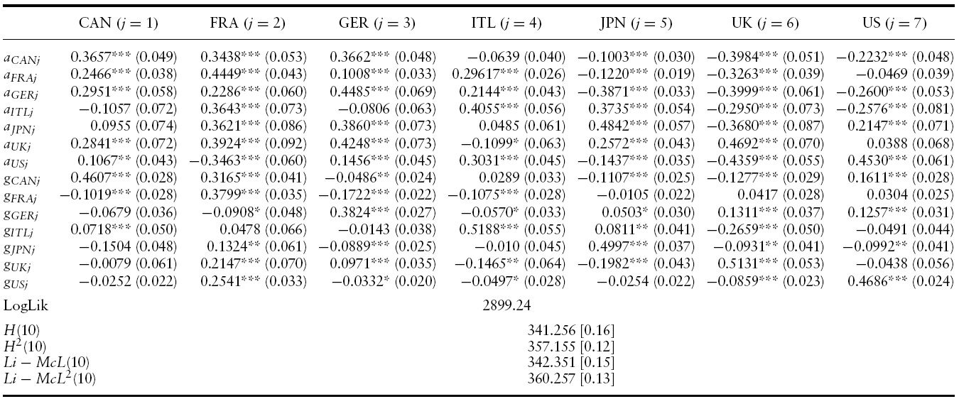
Conditional variance results of VAR(4)-BEKK-GARCH(1,1) model for GDP growth in the G7: 1985Q1?2010Q4
Moreover, the main diagonal elements of the ARCH and GARCH parameters are consistently higher than the off-diagonal ones suggesting that own-country innovation and volatility spillovers are stronger than cross-country innovation and volatility spillovers, respectively.
Our specifications do not suffer fromserial correlation or further ARCHeffects according to Hosking (1980) and Li and McLeod (1981) tests on standardized and squared standardized residuals.
3.4 Volatility Impulse Responses
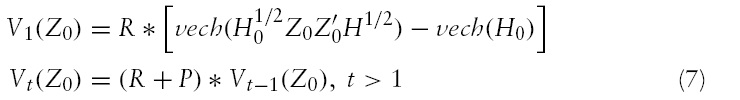
A question that arises and which is of great importance is how rapidly and to what extent a volatility shock in a goods market in the G7 is transmitted to the volatility of the remaining others after a shock occurred. In order to answer that, we follow Hafner and Herwartz (2006) and calculate volatility impulse response functions (VIRF) based on an alternative representation of the BEKK model. Specifically, the vech-representation of the BEKK model introduced by Engle and Kroner (1995) is given by:

where
Assume that at time

where the elements of

It is essential to mention that the VIRFs depend on the initial volatility state,
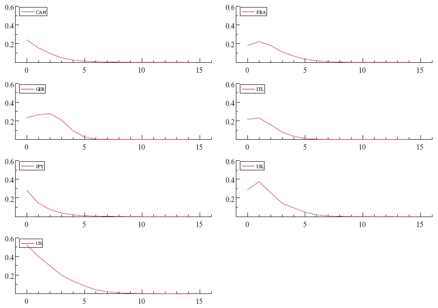
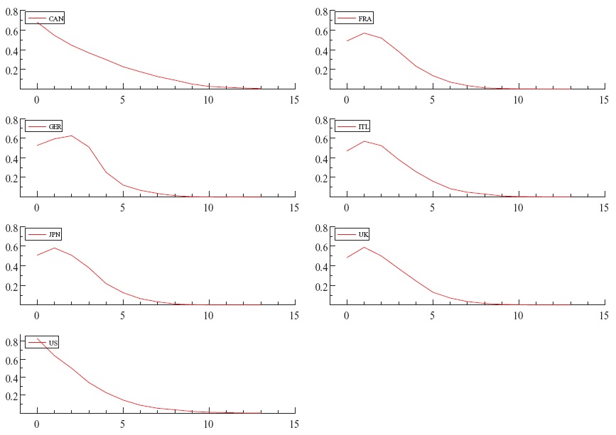
Figures 4 and 5 present the VIRFs for 14 quarters after the 1973 and 2008 crisis.9 Comparing the VIRFs, one can observe that the magnitude and duration of spillovers of the most recent crisis is higher on the volatility of the G7 countries compared with that of the 1973 crisis (the crisis in the 1970s following the first oil price shock). On average, volatility spillovers disappear seven quarters after the 1973 shock and ten quarters after the 2008 shock, respectively. Given the fact that the G7 countries’ initial volatility states in 1973 and 2008 were fairly similar, we conjecture that the difference in their impulse responses is due to the increased goods and financial markets integration in recent years.10
44All estimations are made using RATS Version 7.20. 55The negative values can be attributed to a de-synchronization effect or to a misspecification in the estimation, e.g. a structural break, which we explore below. 6Our results are robust to different transformation of the GDP growth, such as the band-pass filter. 7Even though the latest recession is included in the post-1985 period sample, the results recorded below are qualitatively similar to the post-1985 period ones with the latest recession excluded from the sample. Results of the latter can be provided from the authors upon request. 8The chronology of business cycles used is based on NBER and CEPR. Accordingly, we date the beginning of the recession after the oil-price shocks to 1973Q3 and the beginning of the recent crisis to 2007Q4. 9For the sake of brevity, we only present the VIRFs of the conditional variances. The VIRFs of the conditional covariances can be provided from the authors upon request. 10We also considered several cases of randomly dated shocks in the two subsample periods and obtained similar results.
This paper examines the international spillovers of GDP growth and GDP growth volatility among the G7 countries over the period 1960–2010. The multivariate generalized autoregressive conditional heteroskedasticity (MGARCH) BEKK model of Engle and Kroner (1995) is employed along with volatility impulse responses to identify the source, duration and magnitude of GDP growth and GDP growth volatility spillovers. The results indicate the presence of positive own mean spillovers in each country and of mean spillovers among most of the G7 countries, the latter being in line with the fact that business cycles among countries are synchronized with time lags. In addition, the results document significant output growth own-volatility and cross-volatility spillovers, indicating that shocks to output growth in one G7 country affect both output growth volatility in the respective country as well as in the other G7 countries. An additional finding from the volatility impulse response analysis is that the duration of spillover effects appears to have increased over time, from some seven quarters in the 1970s to some ten quarters during the recent crisis.
Even though evidence of asymmetries in output growth volatility spillovers across the G7 countries is reported, those asymmetries were originated from symmetric shocks. An important avenue for future research is to examinewhether asymmetric shocks of output growth exert dissimilar effects on output growth volatility across countries. On similar grounds, an additional avenue, which we leave for future research, is to check whether and how conditional output growth volatility affects output growth. This can be performed under a GARCH-in-mean multivariate framework.