The financial and currency turmoils of the 1990s in many European, Latin-American and Asian countries have called into question the viability of fixed exchange-rate regimes and led to the development of new models on the causes  of currency collapses. We can now identify at least two main theoretical explanations of crises, one based on the view that a collapse is the inevitable outcome of inconsistent macroeconomic policies and the other based on the view that a collapse results from self-fulfilling expectations. According to the so-called ‘firstgeneration’ models of currency crises, if a government finances its fiscal deficits by printing money in excess of money demand growth, while following a fixed exchange-rate policy, a gradual loss of reserves will occur, leading to a speculative attack against the currency that forces the abandonment of the fixed-rate regime eventually (see, for example, Krugman, 1979; Flood & Garber, 1984; Obstfeld, 1986; Calvo, 1987; van Wijnbergen, 1991; Calvo & Végh, 1999).

The ‘second-generation’ models of currency crises, on the other hand, show that the government’s decision to give up a fixed exchange rate depends on the net benefits of pegging; hence, the fixed rate is likely to be maintained as long as the benefits of devaluing are smaller than the costs. However, changes in market beliefs about the currency sustainability can force the government to go out of the peg. For example, if agents expect a devaluation, a speculative attack will start, forcing the government to abandon the peg, since the costs of keeping the exchange rate fixed outweigh the benefits. On the other hand, if agents expect no change in the currency rate the fixed peg will be preserved. Private expectations are self-fulfilling and multiple equilibria can occur, for given fundamentals (see, for example, Obstfeld, 1996; Velasco, 1996; Cole & Kehoe, 1996; Jeanne, 1997; Jeanne & Masson, 2000).1

More recently, the debate about the role played by fundamentals and/or selffulfilling expectations in triggering a speculative attack has been enriched by a new set of models analyzing currency crises in the context of a change in the  expectations of future policy (see, for example, Burnside et al., 2001, 2003, 2004, 2006; Daniel, 2000, 2001; Corsetti & Maćkowiack, 2006; Maćkowiack, 2007; Singh, 2009). According to this view, explanations of crises do not necessarily require a period of fundamental misalignments. All that is needed is that the path of current and future government policies becomes inconsistent with the fixed peg.

This literature typically uses static models, or models with extrinsic dynamics; that is, models where the dynamics of the system come exclusively from current or anticipated future changes in exogenous variables. Such systems are, in fact, always in steady-state equilibrium in the absence of external shocks. This is in contrast to the so-called intrinsic dynamics of the system, where the economy evolves from some initial stationary state due to, for example, the accumulation of capital stock or foreign assets.2 Models with intrinsic dynamics are useful to understand currency crises and to predict the exact time of an attack. They enable us to study the dynamics of relevant macroeconomic variables.

The purpose of this paper is to deal with this kind of dynamics using a modified version of the Yaari (1965)–Blanchard (1985) model. Our approach has three main advantages. First, it allows a ‘nondegenerate’ dynamic adjustment in the basic monetary model of exchange rate determination. Second, it shows that the macroeconomic equilibrium is dependent on the timing of fiscal policies. Third, the current account is allowed to play a crucial role in transmitting fiscal disturbances to the rest of the economy.

Acentral finding of the paper is that a collapse may occur even as a consequence of a temporary tax cut fully financed by future taxes. In particular, following a fiscal expansion, current account imbalances and the expected depletion of foreign assets will lead to a currency crisis, forcing the monetary authorities to adopt a floating exchange-rate regime. This result is in sharp contrast with the existing literature, where monetary or fiscal policies are inconsistent or expected to be inconsistent with the exchange-rate policy. On the other hand, our theoretical results are consistent with the evidence that Asian countries that came under attack in 1997 were those that had experienced larger current account deficits on the eve of the crisis.3

The main conclusion that emerges from our analysis is that crises can occur in a flexible-price, fully optimizing framework, even when both monetary and fiscal policies are correctly designed; that is, when the intertemporal budget constraint of the government is always respected and monetary policy obeys the rules of the game. The crisis, however, is not driven by self-fulfilling expectations, as the collapse results from well-defined dynamics in the fundamentals. From this point of view, the crisis is basically real and is triggered by the macroeconomic adjustment path associated with a consistent and flexible policy rule that, nonetheless, gives rise to the conditions for a run on the central bank’s foreign reserves. The main implication of our model is that the sustainability of a fixed exchange-rate system may require not only giving up monetary sovereignty, but also strongly restraining the conduct of fiscal policy.4

The paper is organized as follows. Section 2 presents the theoretical model. Section 3 describes the dynamics of the model and the time of the speculative attack. Section 4 concludes.

1The partition between first and second generation models is consistent with the classification scheme of currency crises proposed by Flood and Marion (1999), and Jeanne (2000). From this point of view, the so-called ‘third-generation’ models, elaborated to explain the more recent financial turmoils in Asia, Latin America and Russia, are considered extensions of the existing setups that explicitly include the financial side of the economy   2This distinction may be found, for example, in Turnovsky (1977, 1997) and Obstfeld and Stockman (1985).   3For an exhaustive overviewof the economic fundamentals in Asian countries in the years preceding the financial and currency crisis, see Corsetti et al. (1999) and World Bank (1999).   4Similar implications are also found in Cook and Devereux (2006).

Consider a small open economy described as follows.Agents have perfect foresight and consume a single tradeable good. Domestic supply of the good is exogenous. Household’s financial wealth is divided between domestic money (which is not held abroad) and internationally traded bonds. There are no barriers to trade, so that purchasing power parity (PPP) holds at all times, that is P^∗S = P, where S is the nominal exchange rate (defined as units of domestic currency per unit of foreign currency), P is the domestic price level and P^∗ is the foreign price level. There is perfect capital mobility and domestic and foreign non-monetary assets are perfect substitutes; thus, uncovered interest parity (UIP) is always verified,

where i and i^∗ are the domestic and foreign (constant) nominal interest rate, respectively, and

is the rate of exchange depreciation. In the absence of foreign inflation the external nominal interest rate is equal to the real rate.

The demand side of the economy is described by an extended version of the Yaari–Blanchard perpetual youth model with money in the utility function.5 There is no bequest motive, and financialwealth for newly born agents is assumed to be zero. The birth and death rates are the same, so that population is constant. Let δ denote the instantaneous constant probability of death and β the subjective discount rate. For convenience, the size of each generation at birth is normalized to δ, hence total population is equal to unity.

Each individual of the generation born at time s at each time period t ≥ s faces the following maximization problem:

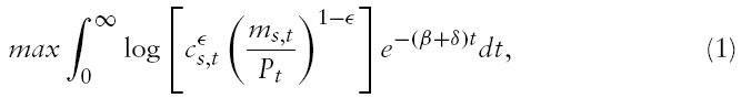
subject to the individual consumer’s flow budget constraint

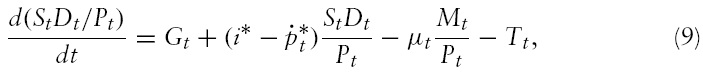
and to the transversality condition

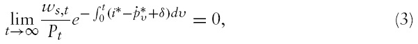
where

6

is the external inflation rate, while c_s, y_s, m_s, w_s and τ_s denote consumption, endowment, nominal money balances, total financial wealth and lump-sum taxes, respectively. Notice that the effective discount rate of consumers is given by β + δ, where

7 Each individual is assumed to receive for every period of her life an actuarial fair premium equal to a fraction δ of her financial wealth from a life insurance company operating in a perfectly competitive market. At the time of her death the remaining individual’s net wealth goes to the insurance company. For simplicity, both the endowment and the amount of lump-sum taxes are age-independent; hence, individuals of all generations have the same human wealth. In addition, the endowment is assumed to be constant over time.

The representative consumer of generation s chooses a sequence for consumption and money balances in order to maximize equation (1) subject to equations (2) and (3) for an initial level of wealth. Solving the dynamic optimization problem and aggregating the results across cohorts yield the following expressions for the time path of aggregate consumption, the portfolio balance condition, the aggregate flow budget constraint of the households and the transversality condition, respectively:

where, η; ≡ (1 − ξ )/ξ . The upper case letter denotes the population aggregate of the generic individual economic variable. For any generic economic variable at individual level, say x, the corresponding population aggregateX can be obtained as

Letting B denote traded bonds denominated in foreign currency, total financial wealth of the private sector can be expressed as:

where we have used the PPP condition.

The public sector is viewed as a composite entity consisting of a government and a central bank. Let D denote the net stock of government debt in terms of foreign currency given by the stock of foreign-currency denominated government bonds (D_G) net of official foreign reserves (R), that is D = D_G − R. Under the assumption that government bonds and foreign reserves yield the same interest rate, the public sector flow budget constraint can be expressed as:

where G is public spending, μ is the growth rate of nominal money and M ≡ M^H + SR with M^H being the domestic component of the money supply (domestic credit) and SR is the stock of official reserves valued in home currency. Henceforth, without loss of generality we assume that G_t = 0.

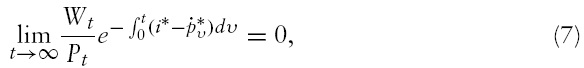
Subtracting equation (9) from equation (6) yields the current account balance:

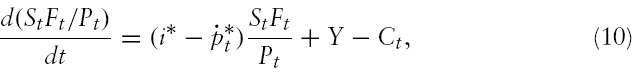
where F = B − D is the net stock of the external assets of the economy. Since D = D_G − Rthe net stock of external assets can also be expressed as F = B + R − D_G.

In order to close the modelwe need to specify the fiscal and the monetary regimes. The government is assumed to adopt a tax rule of the form:

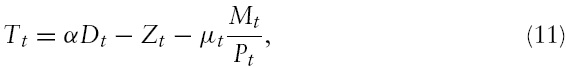
where Z is a transfer and

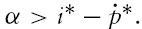
Taxes are an increasing function of net government debt adjusted for seigniorage.8 The parameter restriction on α rules out any explosive paths for the public debt.

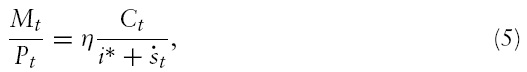
The monetary regime is described by a fixed exchange-rate system. The central bank pegs on each date t the exchange rate at the constant level

standing ready to accommodate any change in money demand in order to keep the relative price of the currency fixed; that is, to accommodate any change in money demand by selling or buying foreign currency bonds. Thus, money supply is endogenously determined according to equation (5) for a given

Under a permanently fixed exchange rate,

and the domestic price level is

The foreign price P^∗ is assumed constant and normalized to one. It follows that

that

By combining equations (4) and (5) with equations (8)–(11), under the fixed exchange-rate regime, the macroeconomic equilibrium of the model is described by the following set of equations:

given the initial conditions on net public debt, on official foreign reserves, on the stock of foreign assets and on nominal money balances: D₀ = 0, R₀, F₀ and M₀. The last term of equation (12) results from the redistribution of financial wealth across generations. If the probability of death δ were equal to zero, the economy would collapse into the standard infinitely-lived representative agent model.9

The dynamic system described by equations (12)–(14) consists of one jump variable (C) and two predetermined or sluggish variables (D and F). The system must have one positive and two negative roots in order to generate a unique stable saddle-point equilibrium path. In the Appendix it is shown that this condition is always satisfied.

5The approach of entering money in the utility function to allowfor money holding behavior within a Yaari–Blanchard framework, is common to a number of papers including Spaventa (1987), Marini and van der Ploeg (1988), van der Ploeg (1991), and Kawai and Maccini (1990, 1995). Similar results could also be obtained by use of cash-in-advance models (see Feenstra, 1986). For aYaari–Blanchard model with cash-in-advance, see Petrucci (2003).   6Following Blanchard (1985), this condition ensures that consumers are relatively patient, in order to ensure that the steady state-level of aggregate financial wealth is positive.   7This assumption ensures that savings are decreasing in wealth and that a steady-state value of aggregate consumption exists. See Blanchard (1985) for details.   8Similar fiscal rules are frequently adopted in the literature. See Benhabib et al. (2001) among others.   9However, for δ = 0 model stability requires that β = i∗.

In this section, we examine the dynamic effects of fiscal policy on the macrovariables of the model to derive the links between future budget deficits and currency crises in a pegged exchange-rate economy. The policy is centered on an unanticipated lump-sum tax cut; that is, a once and for all increase in Z.10 There is a fiscal deficit at time t = 0, generated by the tax cut, followed by future surpluses as debt accumulates, so as always to satisfy the intertemporal government budget constraint without recourse to seigniorage revenues. For the sake of simplicity it is assumed that up to time zero the economy has been in steady-state.

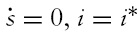
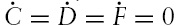
According to Salant–Henderson’s criterion, the peg will be abandoned when the shadow exchange rate, i.e. the exchange that would prevail in the economy in a flexible exchange rate regime, is equal to the prevailing fixed rate. The hypothesis of perfect foresight implies that traders will exchange domestic currency for foreign currency before reserves run out in order to avoid capital losses. The flexible exchange-rate regime that follows the fixed-rate regime’s collapse is assumed to be permanent. For the sake of simplicity, we assume that following the collapse the monetary authorities will adopt a monetary targeting regime characterized by a zero-growth rate of the money, that is

Since the analysis is based on the assumption of perfect foresight, the transitional dynamics of the economy depend on the expectations of the long-run steady-state relationships.

The steady state equilibrium is described by the set of equations (12)–(14) when

and the portfolio balance condition (15). Let

and

denote the long-run levels of consumption, public debt, net foreign assets and real money balances, respectively. The Appendix shows that the long-run effects of a tax cut are described by the following set of derivatives:

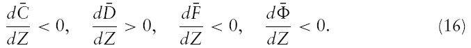
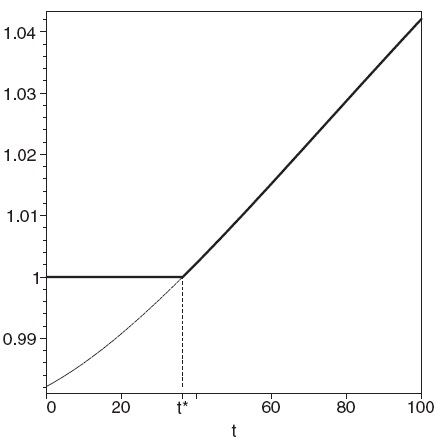
From the above relationships we can see that a tax cut implies that in the new steady-state equilibrium consumption, real money balances and foreign assets are below their original levels, while the government debt is higher.11 Also, notice that the tax cut would imply a jump in consumption (through the wealth effect) and hence an increase in real money balances at t = 0. Given the fixed nominal exchange rate

the increase in real money balances is accomplished by a rise in the nominal money supply. This occurs as households accommodate any changes in money demand with portfolio shifts from foreign bonds to money (i.e., by  selling foreign bonds to the central bank for domestic money). Hence, foreigncurrency assets at the central bank rise on impact, whereas the net stock of the economy external assets goes unchanged as the adjustment in B and R net out in the aggregate. Thereafter, following the contraction in consumption and real money demand along the transitional path, a reverse portfolio shift occurs, as households force the central bank to sell off their reserves for domestic money. Therefore, the model implies that the rise in the budget deficit at t = 0 generates a continuous depletion of foreign assets (or current account deficits) along the transition to the newsteady-state equilibrium, thus making the central bank open to speculative attacks.12 As shown below, this may indeed happen if the shadow exchange rate crosses the pegged rate at some point in time along the economy’s adjustment path. At the time of the attack there will be a jump increase in net government debt and a decline in both net foreign asset and money supply.13

In order to analyze the adjustment of the economy to the initial tax cut, when the public anticipate the collapse of the exchange-rate regime at some point in the future,we need to proceed backward in time. In particular,we first solve the model under the floating exchange-rate regime and find the exact time of the attack, say t^∗. We can then use the results to solve the model under the fixed exchange-rate regime, that is, for 0 < t < t^∗. Notice that perfect foresight requires that all jump variables be continuous at t = t^∗.

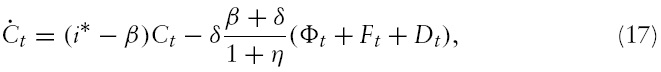
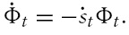
Consider first the model under the floating regime, which applies for t > t^∗. The relevant equations of the system are equations (13)–(14) together with:

where Φ = M/S. Since under the floating regime it is only the exchange rate that responds to variation in money demand, we have that all the observed changes in the level of real money balances are due to changes in the exchange rate, that is

From equation (5), equation (18) immediately follows. Notice that the system of equations describing the economy under the peg (12)–(14) and under the float (13), (14), (17) and (18) have the same steady-state solution, that is

and

As shown in the Appendix, the system of differential equations (13), (14), (17) and (18) is saddle path stable. The solution can be easily obtained by using the initial conditions on the predetermined variables, D, F andM, under a zero level of official reserves. In this way, it is possible to compute the time path for the floating exchange rate before and after the speculative attack. According to the Salant–Henderson criterion, the currency crisis will occur at the point where the shadow exchange rate (i.e., the exchange rate that would prevail in the economy after the fiscal expansion under a flexible regime if the official reserves had fallen to zero) is equal to the fixed rate, that is

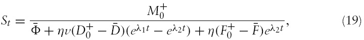
The time path of the shadow floating rate is given by (see the Appendix):

where

and

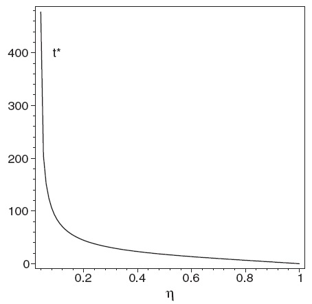
Using the above result and imposing the condition

one can compute the time of the speculative attack. Clearly, the time of the attack also depends on the size of δ. The larger δ, the sooner the crisis will occur. For δ = 0 instead the initial fiscal expansion will not give rise to any change in consumption, in money demand and in the current account, so that equation (19) will become an identity.

After the attack the current exchange rate will depreciate, steadily converging toward a steady state value whose level crucially depends on the initial tax cut:14

where Δ ≡ (α − i^∗)(β + δ − i^∗)(i^∗ + δ)i^∗ > 0. Of course the attack will take place only if the initial tax cut is sufficiently large to bring about a depreciation of the shadow exchange rate such that at a certain point

By contrast, the crisis will not take place if the shadow exchange rate converges towards a level below the peg, that is if

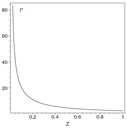
It can be easily shown that the currency crisis will occur only if the initial tax reduction Z satisfies the following condition:

The lower the probability of death δ, the larger the initial tax cut able to trigger a crisis.15 Similarly, we can compute the critical level of the initial stock reserves. For a given Z, speculators will attack the domestic currency only if the level of the initial stock of reserves is such that:

It can be shown that the critical threshold level of initial reserves is increasing in the probability of death δ.16 Proceeding backward in time, it is now possible to describe the time path for the economy under the fixed regime immediately after the fiscal expansion by solving the system of differential equations (12)–(14), given the initial conditions on the predetermined variables, and by imposing the condition associated with the assumption of perfect foresight,which requires that consumption be continuous at the time of the attack t^∗. The analytical solutions are described in detail in the Appendix.

The adjustment process can be better described by making use of a simple numerical example.17

Consider Figures 1–4 and assume, for example, an unanticipated tax cut at t = 0. Figures 1 and 2 plot the current time paths for consumption and the nominal exchange rate (bold lines) and for their related ‘shadow’ levels before the attack occurring at time t^∗. There is, on impact, an increase in consumption, while the shadow exchange rate, after the initial appreciation, starts depreciating steadily.

Current generations profit from the lump-sum tax cut, since they share the burden of future increases in taxation with yet unborn individuals.

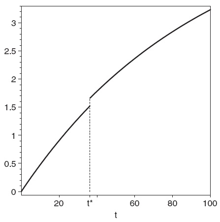
The dynamics of net foreign assets is depicted in Figure 3. Following the tax cut, the economy starts reducing its holding of foreign assets to finance the higher consumption level along the transitional path. Agents accommodate additional money needed for consumption by selling initially B_t forM_t at the central bank’s window. Next, as consumption and real money holdings decline, they exchange domestic money for foreign reserves, using up foreign-currency assets at the central bank. At time t^★ there is an abrupt decline in net foreign assets as a consequence of the speculative attack and the depletion of remaining official reserves. The peg is abandoned and the economy shifts to a flexible exchange-rate regime, where the money supply is under the control of the monetary authorities adopting a simple targeting rule, as already mentioned, foreign assets decline towards the new long-run equilibrium, and the nominal exchange rate depreciates until the current account is brought back in equilibrium.

Figure 4 plots the time path for net government debt, which increases gradually and at the time of the attack jumps upward because of the sudden exhaustion of official reserves, and then continues increasing converging to a new long-run equilibrium above its starting level.

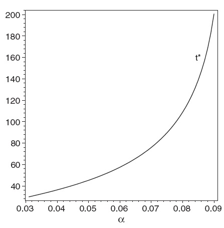
Under the baseline calibration, Figures 5–8 show how the time of the attack t^∗ is affected by the initial level of reserves R₀, the amount of the tax cut Z, the responsiveness of taxes to public debt α and the liquidity preference parameter η;, respectively.The time of the attack depends positively on the level of official foreign reserves and on the responsiveness of taxes to public debt α, but negatively on the magnitude of the fiscal expansion and on the liquidity preference parameter.

Notice that in this model a crisis may occur even when the fiscal budget is showing a surplus.18 This is because, along the transitional path, a sequence of fiscal surpluses will replace the initial sequence of deficits in order to satisfy the government intertemporal budget constraint.

10The effects of government deficit in optimizing models can be found, for example, in Frenkel and Razin (1987), Obstfeld (1989), Turnovsky and Sen (1991).   11It can be easily shown that if δ = 0, the long-run effects of the fiscal expansion will simply be:  That is because when the probability of death is equal to zero, the Ricardian equivalence is restored and the time profile of lump-sum taxes does not affect consumption. In such circumstances a tax cut will not give rise to any current account imbalances and to any change in demand for real money balances, that is why the currency crisis will not take place.   12Strong empirical support for a positive relationship between the current account deficit and current and expected future budget deficits is found by Piersanti (2000). See Baxter (1995) for a more general discussion on this issue.   13Clearly, since movements in fundamentals and hence the speculative attack are predictable in this model, the government could avoid the sharp loss in reserves by abandoning the peg just before  the attack. However, if the government did so, then speculators would incorporate this into their strategies, so introducing strategic interactions and uncertainty into the time of collapse.We do not  consider these issues here, which would terribly complicate the model and make it intractable (as there is no equilibrium in pure strategies) without adding anything newto the Pastine’s (2002) results; nor we consider the optimal exit time issue as in Rebelo and Végh (2006), which nonetheless also involves strategic interactions.We simply focus on the less intricate and narrow target of describing the macroeconomic adjustment path associated with a consistent and more flexible policy rule – in contrast to those considered in the existing literature – which gives rise to the possibility, but not the certainty, of a currency crash, i.e., on the conditions for an attack.   14Recall that under under the floating regime all the observed variations in the level of real money balances are only due to changes in the exchange rate.   15Letting Z∗ denote the critical level of the tax cut above which the peg will collapse, it can be easily shown that     16Letting R*0be the critical stock of reserves below which the crisis will occur, we have that    17Figures 1–4 illustrate a numerical example based on the following parametrization: i∗ = 0.03, η; = 0.25, δ = 0.02, α = 0.04, Y = 1,G = D0 = 0,   F0 = 0.5 and R0 = 0.2. The rate of time preference, β = 0.024, and the initial stock of nominal money balances, M0 = 8.46, are implied. The fiscal expansion consists of an increase in Z of 0.05 from zero.   18This result is consistent with the evidence that in most Asian countries, during the years preceding  the crisis, fiscal imbalances were either in surplus or in modest deficit. See World Bank (1999).

In this paper we have used an optimizing general equilibrium model with overlapping generations to investigate the relation between fiscal deficits and currency crises. It is shown that a rise in current and expected future budget deficits  generates a depletion of foreign reserves, leading up to a currency crisis.

Crises can thus occur even when policies are ‘correctly’ designed; that is, a monetary policy fully committed to maintaining the peg and the fiscal authorities respecting the intertemporal government budget constraint. The sustainability  of fixed exchange-rate systems may thus require not only giving up monetary sovereignty but also imposing a more severe degree of fiscal discipline than implied by the standard solvency conditions.

The authors are very grateful to two anonymous referees for their extremely useful suggestions. The authors also wish to thank Fabio C. Bagliano, Marianne Baxter, Leonardo Becchetti, Anna Rita Bennato, Lorenzo Bini Smaghi, Giancarlo Corsetti, Andrea Costa, Alberto Dalmazzo, Bassam Fattouh, Laurence Harris, Fabrizio Mattesini, PedroM. Oviedo, Alessandro Piergallini, Cristina M. Rossi, Pasquale Scaramozzino, Salvatore Vinci and participants at the II RIEF Conference on International Economics and Finance – University of Rome ‘Tor Vergata’ for helpful comments on previous versions of this paper. The financial support of the MIUR (Grant No. 2007P8MJ7P_003) is gratefully acknowledged. The usual disclaimer applies.