A clear characteristic of the world economy for nearly two decades is the emergence of huge external imbalances (net foreign asset positions) among the major economic areas: the United States has become a large net foreign debtor, and China, Japan, and oil-exporting countries are net foreign creditors in the world economy (IMF, 2006, p. 74; IMF, 2008, p. 35). Despite a contraction of global imbalances in 2009 due to financial crisis, global imbalances are likely to persist also after the recovery due to domestic and systemic distortions (Blanchard & Milesi-Ferretti, 2009; Haldane, 2010) . This is also confirmed by changes in current account positions, which have started to widen again (de Mello
In light of these recent empirical observations, the ‘old’ theoretical question of the impacts of public debt expansion in an interdependent world economy becomes relevant again, albeit under new characteristics of the world economy.1 In contrast to the 1980s, when the spill-over effects of unprecedented levels of US budget deficits under the Reagan administration on countries with a similar production technology (i.e. European economies) aroused concern (Feldstein, 1986), nowadays the world economy is characterized by significant technological differences between advanced and emerging countries. For example, Bai and Qian (2010) report a nearly 50% production share of capital in China while according to, for example, Caselli and Feyrer (2007), the US share is below 30%.2 Moreover, in the late 1980s theworld economy entered a phase of dynamic efficiency (i.e. the world real interest rate was larger than the world GDP growth rate). In the first decade of the twenty-first century, the world economy was almost at the Golden Rule before the financial crisis, since then dynamic inefficiency has prevailed (IMF, 2011, p. 212).
In order to show how these country differences and dynamic (in)efficiencies matter for the economic and welfare effects of unilateral debt expansion (such as prior to and during the financial crisis in the United States),we reconsider in a twogood overlapping generations (OLG) model, with two countries interconnected through trade in commodities and government bonds, the theoretical relationship between a unilateral public debt expansion, the terms of trade and domestic and foreign welfare.3 One finding in the literature dealing with the effects of public debt expansion among similarly developed countries and under dynamic efficiency of the world economy (as characteristic for the 1980s) is that both the terms of trade as well as the welfare effect depend on the net foreign asset position of the involved countries (Frenkel & Razin, 1986; Persson, 1985). If the debt-expanding country is a net foreign creditor and the world economy is dynamically efficient, the gain to future generations from the interest effect may be large enough to outweigh other burdens caused by the debt increase.
In the twenty-first century, two newquestions arise: howrobust are these results for terms of trade and welfare when the economies under consideration are not two equally developed countries but differ in their capital production shares due to different stages of development? And how do these results, obtained for the case of dynamic efficiency, alter when the Golden Rule and dynamic inefficiency are also considered, since the latter reflect better the current situation of theworld economy?
To answer these questions, we will start by analyzing the terms of trade effect of a public debt expansion in a two-country world economy. The terms of trade effect has already been addressed by Zee (1987) and Lin (1994) by extending Diamond’s (1965) one-good, closed economy OLG model with internal public debt towards two countries and two goods. Both authors find that the steady-state effects of public debt on the terms of trade can be positive or negative depending, according to Zee (1987), on the net foreign asset position, or, according to Lin (1994), on the differences with respect to capital production shares (production technologies) between the domestic and the foreign country. In view of these controversial theoretical results and the recent empirical relevance of international technological differences and the dynamic (in)efficiency of the world economy, it is therefore the first objective of this paper to set up a two-good, two-country Diamond-type OLG model, where countries differ in their capital production shares, and to delineate the contribution of internationally technological differences and dynamic (in)efficiency for the terms of trade effects of a public debt expansion.
Given that either positive or negative terms of trade effects may emerge, an obvious question refers to the resulting domestic and foreign welfare effects of unilateral debt expansion (Zee, 1987). Going back as early as Diamond (1965), the welfare effect of a public debt expansion was found negative for the closed economy under dynamic efficiency. In an open economy, one-good framework, however, Persson (1985) shows that even under dynamic efficiency domestic welfare might increase if the debt expanding country is a net creditor to the world economy (if she has a positive external balance or negative net foreign asset position). While these contradictory results were derived in either a closed economy or an open economy one-good framework (where by definition terms of trade effects on overall welfare are excluded), we investigate analytically in our twogood, two-country Diamond-type OLG model Zee’s (1987, p. 603) conjecture that a favorable terms-of-trade effect might lead to a positive welfare impact. The present paper thus derives the domestic and foreign welfare effects of a unilateral debt expansion and identifies the conditions for a positive domestic and/or foreign welfare effect. A special focus lies again on differences in capital production shares across countries and the dynamic (in)efficiency of the world economy vis-à-vis the sign of the net foreign asset position of the debt expanding country
The present paper contributes to the existing literature in the following ways. First, we present sufficient conditions for the existence and saddle-path stability of non-trivial steady state solutions in a two-country, two-good OLG model with country-specific Cobb-Douglas production technologies. Second, we show that the steady state impacts of unilateral public debt shocks on the terms of trade depend on the difference between the domestic and foreign capital production shares and on the dynamic (in)efficiency of the world economy. Third, we demonstrate how the domestic and foreign welfare effects of larger government debt in one country are conditional on the relative magnitude of the capital production shares and on her net foreign asset position as well as on the dynamic (in)efficiency of the world economy.
This paper is organized as follows. In the next section, the structure of the twogood, two-country OLG model with log-linear preferences and Cobb-Douglas technology is described, and the equilibrium dynamics is derived. Section 3 is devoted to the analysis of the existence and dynamic stability of the steady state solutions, and the comparative steady state effects of a public debt expansion are analyzed. In Section 4, we embark on the theoretically interesting case of initially zero public debt levels to illustrate our comparative steady state results. In Section 5, thewelfare effects inHomeand Foreign of a unilateral debt expansion in Home are investigated. Section 6, summarizes the key results and concludes.
1Obviously, this theoretical question is worthwile investigating only if it is empirically warranted. While Meese and Rogoff (1983) illustrate in their seminal paper that movements of exchange rates are best described by a random walk, i.e. there is no systematic relationship between public debt and (real) exchange rates (the real exchange in a two-country world is equal to the inverse of the terms of trade), Gourinchas and Rey (2007) challenge this conclusion by howing that exchange rate movements are instead systematically associated with both future changes of the trade balance (trade channel) and the value of foreign assets of domestic residents relative to their liabilities to foreigners (valuation effect). As early as 1992, Gosh (1992) addressed in an infinitely lived agent (ILA) model with distortionary taxes the latter valuation effect of government expenditures on the external balance. 2This difference is puzzling given the finding that capital shares are in general higher in industrialized countries than in less developed ones (Durlauf & Johnson, 1995) Durlauf aswell as Gollin’s (2002) argument that differences in shares between industrialized and developing countries result from incorrect data treatment of self-employed labor. Note, moreover, that there is a considerable strand of literature showing that aggregate factor shares are not constant over time (for a review, see for example Jones, 2003; Oduor, 2010) 3As argued, for example, by Persson (1985, pp. 82–83), the dynastic savings hypothesis underlying ILA models is theoretically restrictive and poses empirical problems that are avoided by an OLG framework with finitely lived households who do not care for subsequent generations at all (no bequest motive). As a consequence, Ricardian equivalence does not hold and thus changes in public debt affect the terms of trade and welfare in our model.
Consider an infinite-horizon world economy consisting of two countries, named Home and Foreign, which have equally sized working populations
whereby
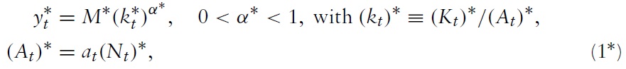
Each country is composed of perfectly competitive firms and households living for two periods. Consumers of both countries have identical preferences, but production technologies are dissimilar across countries to allow both for diverging production shares of factors and total factor productivity. As an extension of Diamond’s closed economy OLG model with neoclassical production into a two-good, two-country setting,we assume constant returns-to-scale technologies that are specified as Cobb-Douglas production functions. As a consequence of constant returns to scale, only per-efficiency-employee variables matter.
To produce the quantity of output per efficiency employee

whereby
In Foreign, the quantity of output per efficiency employee

is produced by employing capital services per efficiency employee

scaled by
Profit maximization in Home and in Foreign imply:


where

denotes the real price of capital services in Home (Foreign) and

is the real wage rate in Home (Foreign).
Without loss of generality, the rate of capital stock depreciation can be set at one, enabling investment of the current period to formnext period’s capital stock. Denoting real investment in capital by

capital thus accumulates over time as follows:

As usual in the Diamond-typeOLGframework, two generations of homogeneous individuals overlap in each period

in return. Domestic aswell as foreign households choose between consumption of domestic,

and of foreign commodities,
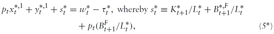
The budget constraint (in real and per-capita terms) of the household living in Home, when young is
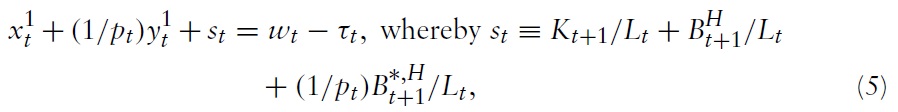
and when old is
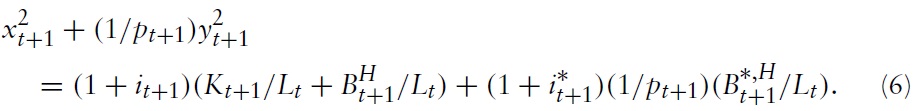
Hereby,

denotes the stock of domestic (foreign) government bonds that the household of Home plans to hold at the beginning of period
Home households’ preferences are represented by the following intertemporal log-linear utility function:

whereby 0 <
The corresponding budget constraints for the household in Foreign are:


denote the stock of domestic and of foreign government bonds that the household of Foreign plans to hold at the beginning of period
Due to the assumption of identical preferences across countries, the utility function of the household in Foreign is:

Government bonds are assumed to be perfectly mobile across Home and Foreign. Hence, a real international interest parity condition holds between the two countries:

Both governments collect lump sum taxes

to finance the costs of perefficiency capita public debt,


where
In line with Diamond (1965, p. 1137), it is assumed that both governments pursue a ‘constant stock’7 budget policy, i.e. they hold the stock of public debt per (efficiency) capita constant over time (see for more details Azariadis, 1993, p. 319, or De la Croix & Michel, 2002, pp. 216–226):

The lump sum tax in both countries becomes endogenous and is determined by

Market clearing of the national labor markets in Home and Foreign requires:

The product market clearing condition of Home reads as follows:
whereas foreign product market clearing demands:
The world market for Home bonds, respectively Foreign bonds, is cleared according to:

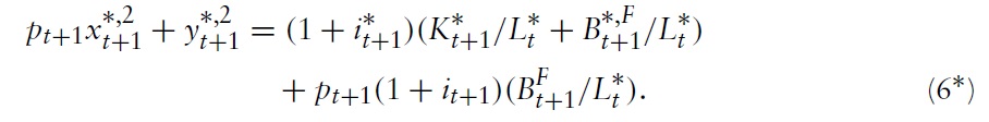
The world asset market clearing condition requires that the total amount of savings in the world equals the total world demand for assets from Home and Foreign:

Due to Walras’ Law one of the market clearing conditions (11)–(14) is redundant.
Having described the optimization problems of households and firms as well as the market clearing conditions, we are now ready to derive the intertemporal equilibrium dynamics.
From the international interest parity condition (8), the equation of motion for the terms of trade follows:

By inserting the optimal saving function for Home

into the world asset market clearing condition (14) and considering the profit maximizing conditions (2) and (3) as well as the equations for lump sum taxes (equations (10)), we obtain the following difference equation describing the law of motion for the international asset market:
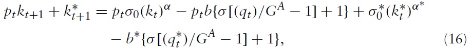
where

are exogenously given.
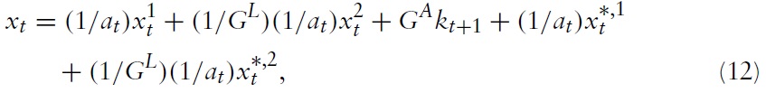
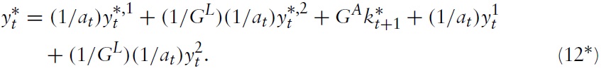
From the two national product market clearing conditions (12) and (12∗), the third dynamic equation is obtained:
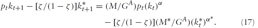
Equations (15)–(17) represent the three-dimensional dynamic system of the twogood, two-country OLG model.
4As usual, stared variables belong to Foreign. 5This assumption represents a deviation of the present model from the assumption of (dynamic) Heckscher-Ohlin models (see Chen, 1992, or more recently Ono & Shibata, 2005). The present model can be regarded as an OLG analogue to Obstfeld’s (1989) and Gosh’s (1992) two-good, two-country ILA models, which the authors use to investigate the current account and terms of trade effects of government expenditures and capital taxes but not of changes in public debt. 6In line with Zee (1987) we assume that equities (i.e. the ownership claims on physical capital) and government bonds are perfectly substitutable and perfectly internationally mobile. 7The alternative to a constant-stock budget policy is to hold a flow, such as the net or the primary deficit, constant over time. Such a budget policy is termed a constant-flow policy (Azariadis, 1993, p. 322, or De la Croix & Michel, 2002, pp. 193–203)). In viewof the problems of the European Union to cope with the target debt-to-GDP ratio in the Maastricht treaty and of the US to remain below the debt ceiling, a constant stock policy seems to be empirically more relevant.
3. Existence, Dynamic Stability and Comparative Statics of Steady States
3.1 Existence and Stability of Steady States
The first step needed when analyzing the system dynamics of our model is to investigate the existence of steady state solutions,

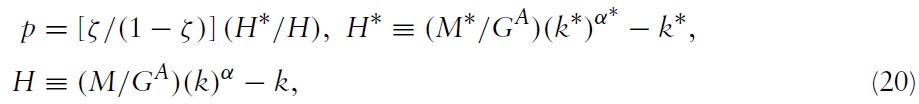
Evaluating equations (15)–(17) at the nontrivial steady state gives:
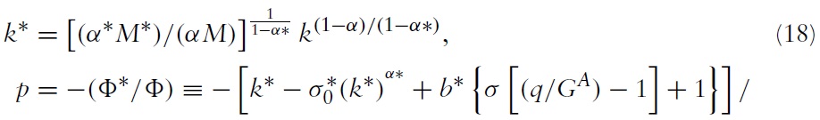


where Φ (Φ∗) in equation (19) denotes the net foreign asset position of Home (Foreign) and
Proposition 1 provides sufficient conditions for the existence of two (one) nontrivial steady states (state).8
Proposition 1


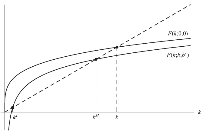
Figure 1 illustrates the main idea behind the proof of Proposition 1. Equating equations (19) and (20) and inserting equation (18) yields
We know from the proof of Proposition 1 that

which would be tangent to the 45◦ line (not shown in Figure 1), and hence there exist two nontrivial steady state solutions
Before proceeding to the comparative statics analysis of a domestic public debt expansion, we investigate the local stability of the non-trivial steady-state solutions by means of linear approximation of the equilibrium dynamics in a small neighborhood of the steady states. In contrast to asymptotic dynamic stability of non-trivial steady states in a closed economy (Rankin & Roffia, 2003, p. 231) or in a one-good, two-country model (Buiter, 1981, p. 787), in a two-good, two-country OLG model only saddle-path stability of the steady states can be obtained. Thus, Proposition 2 claims the saddle-point stability of the steady state with the larger capital intensity.9
Proposition 2

Proposition 2 implies that Zee’s (1987) assumption of asymptotic dynamic stability of the terms of trade dynamics10 cannot be true at least for our loglinear, Cobb-Douglas OLG model. Thus, it is natural to suggest that the Zee-Lin divergence about the steady state effects of public debt changes on the terms of trade can be traced back to Zee’s questionable assumption of asymptotic dynamic stability of external terms of trade dynamics.11
3.2 Comparative Steady State Analysis of Unilateral Shocks in Public Debt
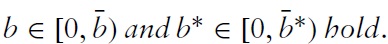
Let us turn nowto comparative steady state analysis of a shock in per-capita public debt in Home in a small neighborhood of the larger k under the assumption that, in order to guarantee that public debt per capita remains sustainable in the long run, the shock is not too large. As shown in Appendix A.3, the steady state effects of a marginal expansion of public debt in Home are given by:
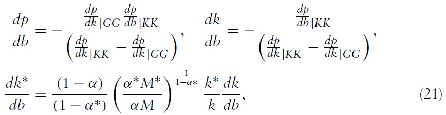
where
Proposition 3
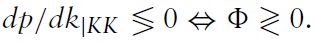


The slope of the KK-curve can be intuitively explained as in Zee (1987, p. 613). To understand why the GG-curve is positively sloped if the capital production share in Home is less than in Foreign, suppose that the terms of trade rise while the capital intensity remains unchanged. Hence, equilibrium condition (20) is violated since the left-hand side exceeds the right-hand side. To restore equilibrium in both commodity markets, the right-hand side of equation (20) has to rise. Since dynamic efficiency implies that the steady state interest factor
In addition for being decisive for the slopes of the curves, the shift of the KKcurve in response of the shock also depends on the net foreign asset position and the capital production shares.When Home is a net foreign creditor, the KK curve shifts upwards, while it shifts downwards when Home is a net foreign debtor, regardless of the dynamic (in)efficiency of the world economy. To understand this shift of the KK-curve, i.e. that the terms of trade increase (decline) when holding Home capital intensity fixed, consider again the case of Home being a net creditor. When the level of public debt in Home rises and
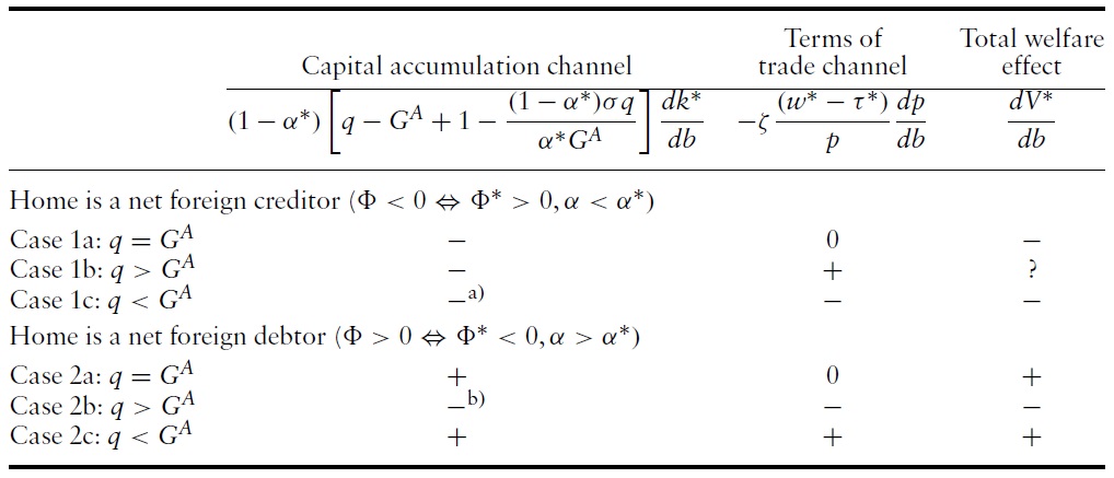
The total effects of marginal changes inHomepublic debt onHomeand Foreign capital intensities and the respective terms of trade are stated analytically in Proposition 4.
Proposition 4
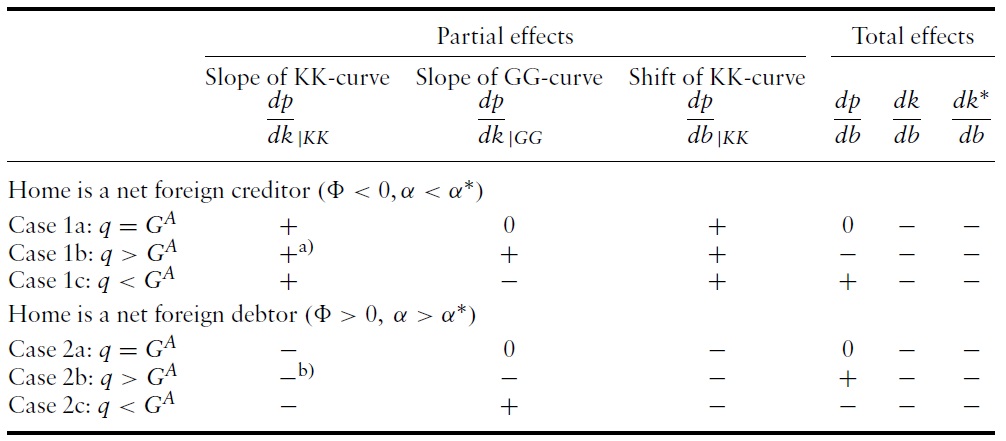
Slopes and shift of the KK- and GG-curve as well as total derivatives for the six cases (for b = b? = 0)

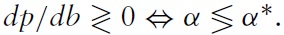
Proposition 4 reveals that in contrast to Zee’s (1987, p. 617) conclusion that ‘a higher level of domestic government debt leads to a fall (rise) in the terms of trade if, at the initial steady state, the home country is a net debtor (creditor)’ the response of Home’s terms of trade to a marginal increase of public debt is exactly opposite.15 More importantly, whether the terms of trade improve or deteriorate, hinges only on the relation between Home and Foreign capital production shares and on the dynamic (in)efficiency of the world economy, but not on the sign of the net foreign asset position. Taking into account Lin’s (1994) definition of the real exchange rate (= the inverse of our terms of trade) as the ratio of Foreign to Home real wage rate and assuming dynamic efficiency, the terms of trade changes – according to case (ii) in Proposition 4 – confirm his results (Lin, 1994, p. 102): if the capital production share in Home is larger (smaller) than in Foreign, Home’s terms of trade improve (deteriorate) with rising public debt in Home.
The intuition behind this result is as follows. Higher public debt in Home lowers Home and Foreign capital intensity, less so in Foreign than in Home, if the production share of capital in Home is larger than in Foreign (see equation (20)).
8The whole spectrum of steady state solutions is characterized in Farmer and Zotti (2010) for internationally equal saving rates and in Farmer (2011) for unequal saving rates but for equal production elasticities of capital. In particular, the upper limits for the domestic and foreign public debt level where only one non-trivial steady state solution occurs is explicitly calculated. 9In log-linear, Cobb-Douglas OLG models, conditions for the existence of steady states often imply dynamic stability as in the closed economy models of Ono (2002) and Farmer and Wendner (2003). 10In general, two approaches to dynamic stability of steady states can be found in the literature (Gandolfo, 1997,p. 334): the first approach adopted by Zee (1987, p. 615) assumes asymptotic dynamic stability as a necessary condition for comparative steady state analysis, the second approach investigates sufficient conditions regarding preferences, technologies and policy parameters for dynamic stability. 11Although Lin (1994,p. 101) uncritically takes over Zee’s (1987) stability assumption, it does not lead him to erroneous conclusions due to his definition of the terms of trade as a non-dynamic variable. 12 Zee (1987, p. 617) assumes a similar restriction which is fulfilled for not too large b/k b∗/k∗). 13Note, however, that the net foreign position is determined endogenously in the model. Thus, all parameters (including the level of public debt) and the endogenous variables p, k, and k∗ determine the countries’ net foreign asset positions. 14It is worth noting that Zee (1987, p. 614) claims that the terms of trade in general equilibrium, i.e. when both k and k∗ adapt to the increase in b, depend on the lending-borrowing status (in our terminology net foreign asset position) of Home. As our analysis shows, the terms of trade depend on the lending-borrowing status of Home only for given capital intensities and not in general equilibrium. Thus, his analysis acknowledges only the shift of the KK-curve dp/db|KK (see fourth column of Table 1). 15This comes at no surprise since Zee (1987) erroneously assumes asymptotic instead of saddle-point stability.
4. Illustrations of Comparative Statics Effects for Initially Zero Debt Levels
Although obviously at odds with current reality, especially in advanced countries, we will employ in the following the special case of
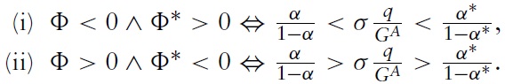
Proposition 5

Proposition 5 is most easily understood for a Golden Rule situation (
To ease understanding of Proposition 5 we will use graphical and verbal explanation of the six cases that emerge when
Starting with the case of the Golden Rule, we see that the slope of the GGcurve at the stationary state is zero (case (i) in Proposition 3), i.e. the GG-curve is horizontal (see upper left diagram in Figure 2). The slope of the KK-curve is determined by the sign of the net foreign asset position of Home: if Home is a net foreign creditor, the KK-curve is positively sloped, and otherwise is negatively sloped. According to case (ii) in Proposition 3, under dynamic efficiency, the slope of the GG-curve depends on the magnitude of Home production share of capital relative to Foreign: the GG-curve is positively sloped if
In addition to being decisive for the slopes of the curves, the shift of the KKcurve in response of the shock also depends on the net foreign asset position.When Home is a net foreign creditor, the KK curve shifts upwards, while it shifts downwards when Home is a net foreign debtor, regardless of the dynamic (in)efficiency of the world economy (see also Table 1). In all cases, the position of the GG-curve is not affected by unilateral constant debt budget policy
Proposition 4 (i) claims that in a GoldenRule situation the resulting steady state effects for the capital stocks are negativewhile there is no terms of trade effect (see cases 1a and 2a in Table 1). As a consequence of dynamic (in)efficiency, the slope of the GG-curve is now positive or negative, depending on the country difference in capital production shares and related net foreign asset position. Thus, in contrast to the Golden Rule situation, there is an additional impact on the terms of trade, which is negative when the GG-curve is positively sloped (cases 1b and 2c) and otherwise positive (cases 1c and 2b). Moreover, regardless of the constellations of slopes of the two curves, the effect on domestic capital stocks is always negative (crowding out), since the KK curve shifts upward whenever it is positively sloped while it shifts downwards otherwise. Because of
16Choi and Mark (2009, pp. 5–6) observe that US and Japanese government budget deficits are only slightly correlated with the current account of these countries. Thus, the authors focus on the implications of savings (and investment) behavior for the external balance, which also plays an important role in this section. 17In the general case of initially positive public debt levels, ten cases emerge according to Proposition 3.
5. Steady State Welfare Effects of a Unilateral Change of Public Debt
Knowing that a public debt expansion by one country leads to a decrease in both Home and Foreign capital stocks but that Home’s terms of trade either increase, decrease or remain fixed (depending on the international difference in capital production shares and dynamic (in)efficiency), it remains to be investigated what these impacts imply in total for welfare in both countries. Methodologically, this section is thus devoted to expanding Diamond’s (1965, pp. 1141–1143) closedeconomy and Persson’s (1985) one-good, two-country welfare analysis into a two-good, two-country setting and by investigating the welfare effects in both countries. We will illustrate how the steady state welfare effects of public debt expansion in our model depend both on the net foreign asset position and dynamic (in)efficiency as in Persson (1985) , and proceeding beyond Persson (1985) we show why steady state welfare of a unilateral expansion of public debt depends essentially on international differences in capital production shares (directly via the terms of trade effect and indirectly via the net foreign asset position).
To derive the domestic steady state welfare effects, we introduce the indirect lifetime utility function

Since, moreover,

Before investigating the sign of the total welfare effect, note that the first term in braces in equation (22) corresponds exactly to the closed economy term of Diamond (1965), which captures the
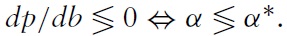
Inspecting equation (22), we see that under dynamic efficiency (
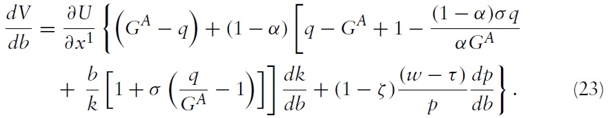
The first term in braces in equation (23) can be termed the
Proposition 6 generalizes the result that Persson (1985, pp. 80–81) obtained for a one-good, two-country world economy into a two-good framework with internationally diverging capital production shares and initially zero public debt levels.
Proposition 6

Starting with the case of the Golden Rule (
Under dynamic efficiency, a net foreign creditor’s welfare effect through both the terms of trade and the dynamic efficiency channel is negative (see case 1b). If, moreover,
Under dynamic inefficiency, debt expansion leads for a net foreign creditor country to an additional positivewelfare effect through the terms of trade channel (see last term in equation (23)), and a direct positive effect through the dynamic efficiency channel (see first term in equation (23)), which reinforce the positive welfare effect through the capital accumulation channel (case 1c). On the other hand, for a net foreign debtor country the terms of trade effect is negative leading to an ambiguous total welfare effect (case 2c).
Our results require a qualification of Zee’s (1987, p. 603) suggestion that ‘the favourable terms of trade effect for the home country, if she is a net creditor, suggests that the likelihood for home consumer’s welfare actually to increase is even higher than in Persson’s one good framework’ – this relationship is only true if Home has a smaller capital production share than Foreign and if the initial steady state is
[Table 2.] Home’s welfare effects for the six cases cases (for b = b? = 0)
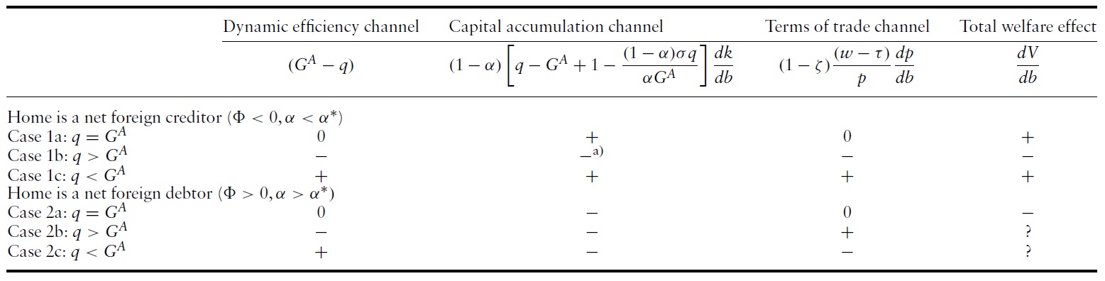
Home’s welfare effects for the six cases cases (for b = b? = 0)
Proceeding similarly as for Home, the Foreign welfare equivalent to equation (22) is:
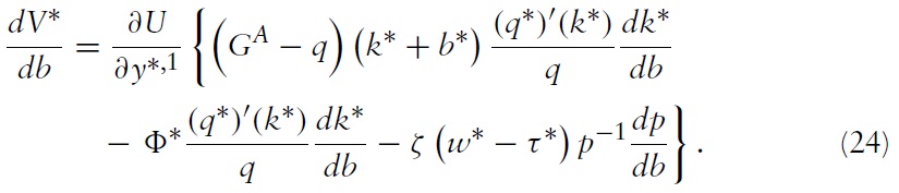
Comparing equation (24) to equation (22) reveals that foreign welfare is affected by a domestic debt expansion only indirectly, such that the intratemporal terms of trade effect (see last term in equation (24)) is in the opposite direction than that in Home and that the wealth effect on Foreign is simpler.
Again, the direction of the effect of Home public debt expansion on Foreign welfare depends on dynamic (in)efficiency (see the first term in braces in (24)), the Foreign net foreign asset position (see the second term) and the terms of trade effect (see the third term). Under dynamic efficiency (
To obtain again an unambiguous overall welfare effect, we rearrange equation (24) into equation (25):
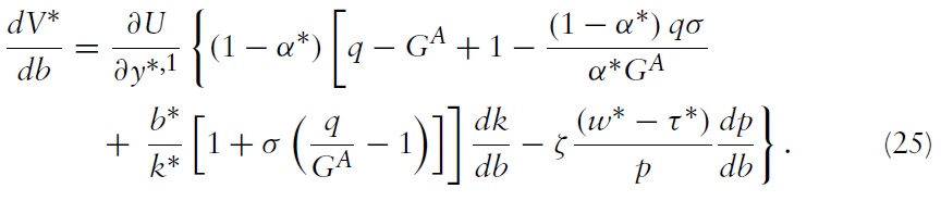
The resulting changes in Foreign’s welfare effects are described in Proposition 7 and Table 3.
Proposition 7
i)
[Table 3.] Foreign’s welfare effect for the six cases (for b = b? = 0)

Foreign’s welfare effect for the six cases (for b = b? = 0)
(ii)
(iii)
In contrast to Home, for
5.3 Welfare Effects for the Illustrative US-China Case
Let us finally discuss the empirically relevant case of the United States and China, where Home has a lower capital production share and is a net foreign debtor country and the world economy is dynamically inefficient (or the Golden Rule applies).21 Since this initial steady state constellation is not compatible with any of the six cases described in Section 4 above,we first showhowthe strict relationship between the external balance and capital production shares isweakenedwhen the debt level in at least one country is sufficiently positive in the initial steady state.
To see this, note that (ii) in Proposition 5 reads for the general case of initially positive public debt levels as:Φ > 0 ∧ Φ∗ < 0 iff1 − [(1 −
Our illustrative empirical example of Home being the United States and China being Foreign corresponds to
18To simplify exposition, we set a = 1 in this section. 19Clearly, if the interest and growth factor difference is smaller than the net foreign asset term, then the Persson result of a positive total welfare effect emerges. 20Note this claim does not hinge on the assumption of b = b∗ = 0. 21One important deviation from reality is however our modeling assumption of internationally equivalent saving rates. This assumption should be relaxed in future research. 22This approximation of foreign (i.e. China’s) debt per efficiency capita is warranted since the debt-to-GDP ratio of China in 2016 is forecast to be 9.7% while the US debt-to-GDP ratio will be 111.9% in 2016 (IMF 2011).
This paper reconsiders the effects of a unilateral expansion of public debt on terms of trade, capital accumulation and welfare in a two-good, two-country OLG model of the world economy with internationally uneven capital production shares. As outlined in the introduction, not only the enhanced empirical relevance but also controversial claims regarding the role of the net foreign asset position and capital production shares versus the dynamic (in)efficiency of the world economy in the established literature justify this reconsideration. Moreover, we were able to close the research gap concerning the welfare effects of unilateral public debt expansion in two-good, two-country OLG models with country-specific capital production shares not only under dynamic efficiency but also for dynamic inefficiency and the Golden Rule.
As a prerequisite for the analysis of terms of trade and welfare effects we performed a thorough analysis of the existence and dynamic stability of steady state solutions.We find that—as in a model with similar capital production shares across countries—two non-trivial steady states of private capital intensities in Home and Foreign exist if the time-stationary (sustainable) public debt levels in both countries remain below some maximum level. The steady state with the larger domestic capital intensity is saddle-path stable—a result that starkly contrasts with the presumption of Zee (1987) that the terms of trade dynamics are asymptotically stable.
Moving on to comparative steady state analysis, we find that under a mild restriction on debt to capital intensity ratios in both countries, capital intensities in Home and Foreign fall in response to higher public debt in Home, albeit for different reasons. The terms of trade effect however differs and its direction depends on the relation between domestic and foreign capital production shares and on the dynamic (in)efficiency of theworld economy: under dynamic efficiency, the terms of trade either improve (when the capital production share in Home is
To disentangle the significance of the net foreign asset position, the capital production share and the dynamic (in)efficiency for the welfare effects of expanded public debt, we focus on the theoretically interesting case of initially zero debt levels. In that case a strict relationship holds between international differences in net foreign asset positions and capital production shares:when the Home country has a larger (smaller) capital production share than Foreign, then Home is a net foreign debtor (creditor) country and Foreign a net foreign creditor (debtor).
Regarding the welfare effects, we verify in our model with internationally diverging capital production shares Persson’s (1985) result that the welfare effect for a net foreign creditor (debtor) country is certainly positive (negative) while it is negative (positive) for the other country when the Golden Rule applies. Clarifying Persson’s (1985) ambiguous findings for dynamic efficiency, we state explicitly under which condition welfare in a debt expanding net foreign creditor country declines: the difference between the interest and the growth factor has to dominate the effect via the positive external balance.
Comparing the welfare effects of domestic debt expansion for Home and Foreign within our model setting, it becomes apparent that only one country can gain by a unilateral debt expansion, but not both. In particular, domestic welfare increases and foreign welfare decreases when Home has a lower capital production share than Foreign (and reversely when Home has a higher share). While this result holds strictly only for the Golden Rule, the result of opposing welfare effects may also emerge under dynamic (in)efficiency where the terms of trade change and impact on welfare. From a worldwide perspective, the welfare loss in one country might exceed the gain in the other country, causing eventually a world-wide welfare decline.
What can we conclude about the significance of pronounced differences in capital production shares and external imbalances across major areas of the world economy for the impacts of unilateral public debt expansion on terms of trade and welfare? Applying our theoretical insights to the empirically interesting case of the United States and China, which is characterized by a smaller capital production share in the net foreign debtor country, we focus on the Golden Rule (as in the decade prior to the financial crisis) and dynamic inefficiency (as in the post crisis period). While in a Golden Rule situation of the world economy, US welfare responds negatively to domestic public debt expansion, and China’s welfare increases in our model context. Under dynamic inefficiency however, US welfare increases when the difference between the growth and the interest factor dominates the effect via the negative external balance. Thus, one is tempted to conclude that the change in dynamic efficiency of the world economy made it easier for US politicians to run levels of public deficits which would have been infeasible prior to the crisis.
This paper can be extended along two lines. First, more general utility and production functions can be used to check the dependence of the results on the particular functional specification. A second fruitful extensionwould be to incorporate uncertainty of risk-averse households with respect to future prices and interest rates in order to arrive at demand functions for physical capital and government bonds instead of indeterminate asset portfolios as in our model. It would be interesting to see how the results we obtained under the assumption of perfectly substitutable capital and bonds change if we start from imperfectly substitutable assets along the lines of Enders and Lapan (1983) or more recently Choi and Mark (2009).