State Trading Enterprises (STEs) are periodically subject to intense scrutiny for their suspected negative impact on the international trade of agricultural goods. Sound empirical assessment of the impact of STEs is scant, in spite of the ongoing and intense debate over their impacts, especially in the context of reform at the WTO. In this paper we use the case of world wheat trade between 2212 country pairs over a 35 year span to assess STE impacts. Using a gravity model, we estimate a Poisson pseudo maximum likelihood fixed effects model of world wheat trade to assess the role of both the presence of STEs and STEs with monopoly power. Further addressing estimation challenges,we also estimate zeroinflated versions of Poisson and Negative Binomial Regression models. We find consistent support for the hypothesis that monopoly export STEs are associated with higher exports for their host country. Similarly, import STEs appear to inhibit wheat imports, suggesting a protectionist function.
State Trading Enterprises (STEs) are fromtime to time subject to intense scrutiny for their suspected negative impact on the international trade of agricultural and other goods. In contrast to private traders, STEs may have special rights and privileges, including mandates and access to public treasuries. Proposals at the World Trade Organization (WTO) advocate that agricultural STEs give up monopoly powers over the import or export of agricultural products, and that benefits such as the ability to have losses covered by their public treasuries be removed. On July 17, 2007 Ambassador Crawford Falconer, chairperson of the agriculture negotiations at the WTO, circulated his 45-page revised draft modalities which call for the elimination of the use of monopoly export powers for STEs by 2013 (Falconer, 2007). The implied assumption is that monopoly power of STEs distorts trade and therefore its removal would lead to increased benefits of international trade in agricultural products.
Exporting STEs are intended to facilitate exports for the benefit of domestic producers and their national economies. Theremay be historical reasons for their use, such as providing logistical support and market information for domestic producers in the development of an industry, or the protection of farmers from perceived predatory practices by large private traders.1 Concerns over the ability of STEs to distort trade extend to import STEs,whichmay be used to limit market access to protect their domestic producers.2 Reasons for import STEs include the ‘infant industry’ argument (for domestic producers), domestic security, and food safety. Regardless of their initial purpose or function, the relevant question in the terms of international trade is whether the presence of STEs confers unfair trade benefits on their host countries. Rigorous and systematic empirical assessment of the impact of STEs on their host county’s imports or exports is necessary to assess the alleged distortion, but is largely absent.
Numerous studies have examined various aspects of specific STEs, including the effect of price pooling, the possibility of price discrimination, and the most applicable market structure framework – monopolistic competition versus oligopoly. Findings are mixed. Import STEs are found to be less responsive to sources of supply when market conditions change, compared with private traders (Abbott & Young, 1999). There is some evidence that exclusive rights of export STEs in the case of the Australian Wheat Board (AWB) do not necessarily lead to an ‘unfair’ advantage in international markets (McCorriston & MacLaren, 2007b; McCorriston and MacLaren, 2007a,b). Further, altering the current roles of STEs will not necessarily lead to increased competition, as market structure responses are likely (Scoppola, 2007). Various classification systems outline the conditions under which STEs are potentially more or less trade distorting (Dixit and Josling, 1997; McCorriston&MacLaren, 2001; Fulton
The relative absence of systematic and rigorous empirical evidence regarding the trade impacts of STEs has a number of fundamental sources. First, STEs vary across countries as well as over time. A clear and consistent definition is essential to resolving the issue of trade distortion. Second, data requirements are onerous in terms of consistent measurement for a large number of variables and across a large number of countries. Third, there are significant empirical issues such as correcting for zero trades, controlling for fixed effects, heteroskedacticity biasing the results, and robustness checks. However, as more trade and country-specific data become available, along with advances in technique, these barriers are not insurmountable. Fixed effects models, for example, are key to isolating the effects of particular trading-country pair attributes, such as the idiosyncratic effects of demand or transportation costs. Further, advances in count-data estimation techniques allowfor more accurate and precise modelling, including the inclusion and proper treatment of zero-trade observations and heteroskedasticity.
In this paper, we assess whether exporting (importing) STEs have an effect on their host country’s wheat exports (imports), controlling as completely as possible for other influences including fixed effects. This study represents the first assessment of the general effect of STEs using trade data across all countries versus the case study approach that predominates this literature. We estimate separately the effect of an STE and a monopoly STE on either the imports or the exports of the host countries.3We use a common data source: the United Nations Commodity Database for data on world wheat trade flows between 180 countries from 1970 to 2005. A gravity model approach is employed using several countmodel estimations that account for fixed effects, as well as to address problems of heteroskedasticity that arise when estimating gravity models using ordinary least squares (OLS). Our approaches allow a rigorous estimation of STE effects and we consider potential problems such as zero inflation (excess zero trades) and over-dispersion in robustness tests. Our results suggest that monopoly export STEs are associated with the enhanced value of wheat exports. Further, although not quite as consistently, the presence of import STEs (without monopoly) is negatively related to wheat imports of the host country. The evidence suggests that the WTO’s focus on STEs as being potentially trade distorting is justified.
This paper is organized as follows. Section 2 is an overview of previous examinations of the role of STEs in theworldwheat trade, followed by an overview of the gravity model approach. Section 4 presents the empirical implementation, with results following in Section 5. Conclusions are offered in Section 6.
1Examples of this type of origin are the Canadian and Australian Wheat Boards. 2An example of an import STE is the Japanese Ministry of Agriculture, Forestry and Fisheries (MAFF), which controls the importation and pricing of wheat. 3We define a monopoly STE as an STE that has been given exclusive marketing rights by the host government.
2. The Role of STEs in Wheat Trade
Agricultural STEs are major players in the world marketplace. For example, the Canadian Wheat Board (CWB) is the largest exporter of wheat in the world (Schmitz&Furtan, 1999).To assess their role,we use the WTO definition of STEs:
[Table 1.] Presence of STE in global wheat STEs from 1970 to 2005
Presence of STE in global wheat STEs from 1970 to 2005
Further, we rely on the (required) notification by individual countries regarding their use of an STE. We acknowledge that this definition still leaves some scope for varying size, structure, power, and government involvement across countries. However, we believe these limitations are outweighed by the fact that this is the operational definition of the WTO, forming the reference point in trade reform, and it is the only common definition across countries.
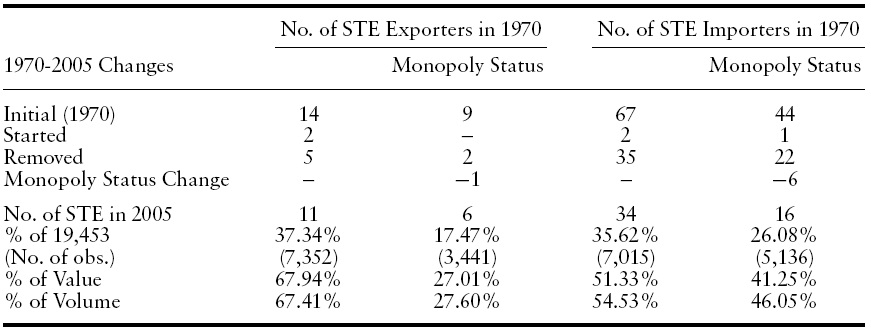
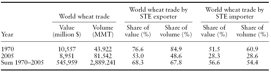
Table 1 shows the importance of STEs in the world wheat trade using the WTO’s definition. Clearly both STE exporters and importers account for a very substantial portion ofwheat value and volume, although their relative importance has declined over the period. Size and market share raise concerns that STEs are anticompetitive, including the possibility that exporter and importer STEs provide a front for protection of domestic agriculture. Further, some governments provide STEs with subsidies, such as lower-than-market rates for capital or subsidies for the price of farm commodities. However, successful challenges at the WTO regarding the use of STEs require sound empirical evidence of their trade impact.
The common theoretical framework for examining the impact of STEs is imperfectly competitive firms in a trade environment as set out by Brander and Spencer (1985) (Hamilton & Siegert, 2000, 2002; Carter & Smith, 2001; McCorriston & MacLaren, 2005, 2007b). In the case of an exporting STE, these models start by assuming the STE purchases the product from farmers and then sells it on the domestic or world market. The complete proceeds from the export sale may or may not be returned to farmers. In the case of STE importers, the STEs purchase the product on the world market and sell it domestically at or below cost. In either case, an STE, and perhaps especially one that is granted a monopoly by its host country, has the potential to exercise market power to the advantage of domestic producers. The particular goals of the STE regarding trade facilitation or a restriction will help determine actual outcomes.
Findings regarding the presence of market power that emerge from the detailed examination of a particular institution, the CWB, are mixed. Schmitz and Gray (2000) found that the CWB was able to capture revenues beyond what would have been generated by purely competitive sellers. This finding is supported by Kraft
Other approaches to assessing particular STEs have consisted of a time-series examination of grain prices (Goodwin & Schroeder, 1991) and a comparison between the distribution effects of price pooling and export subsidies (Alston & Gray, 2000), generally pointing to a positive impact on grain prices. The CWB in particular has been scrutinized in the context of the advantages and disadvantages of a single desk seller (Clark, 1995; Dixit&Josling, 1997). In a more recent study, Dong
Conspicuously absent in the empirical STE literature is an approach that uses a fully specified econometric model of international trade, where the determination of the exercise of market power would rest on the significance of the STE coefficients after fully accounting for other factors, including fixed effects and zero trades. Case studies are useful in a descriptive sense but have serious shortcomings for global comparisons and to make generalizations for policy analysis. This paper addresses this relative vacuum in the assessment of the impact of STEs in the wheat trade. Following from the theoretical frameworks outlined above, we use a gravity model to test two null hypotheses.
The gravity model was first developed to describe trade flows by Jan Tinbergen (1962), even though the analysis and conclusions were strictly intuitive, rather than being theoretical grounded. Since then, the gravity model has been sed extensively in the empirical trade literature. Despite its widespread use and repeated empirical validation, the theoretical micro-foundations of the gravity model have only been established relatively recently, leading to a resurgence of its use (Anderson & van Wincoop, 2003; Sheldon, 2006).
The gravity model has been used in numerous trade theory contexts including monopolistic competition in the new trade theory (Helpman & Krugman, 1985; Helpman, 1987) and variations of the classical Heckscher-Ohlin-Samuelson (HO/HOS) model (Bergstrand, 1985; Deardorff, 1998). Sheldon’s (2006) reviewof the literature shows that the gravity model is an empirical workhorse in assessing the effects of market and institutional structures.4 For example, refinements of the gravity model have been used to test the influence of variables pertaining to current and past policies, geography, common history, and institutional arrangement such as STEs (Rose & Spiegel, 2009; Rose, 2004; de Groot
In its simplest form, the gravity model can be represented as:

The term

where

and

In equation (1),
4Sheldon (2006) shows the gravity model works well empirically for both differentiated and homogeneous goods.
A gravity model is used to investigate bilateral wheat trade values over the 1970–2005 period. One advantage of considering wheat is that it is a relatively homogeneous product.5 In addition to standard gravity model components, a number of additional variables are included to add to the explanatory power of the model and to test our hypotheses surrounding STEs.
In using the gravity model for the study of a particular commodity, several adjustments are required. Most gravity models have been used for the
The conventional log-linear gravity model specification for this analysis would be:
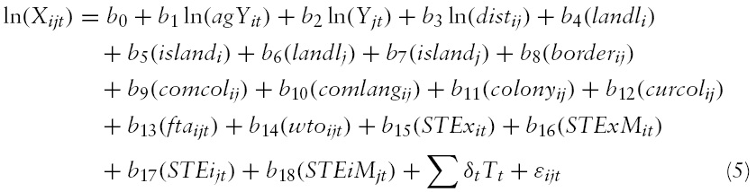
where
Agriculture GDP in the exporting country (
The usual log-linearization shown in equation (5) presents a serious issue in interpreting the gravity equation coefficients due to heteroskedasticity, and in dealing with zero trade flows (representing more than 79% of our 94,716 country-pairs our trade flows). In particular, Silva and Tenreyro (2006) show that estimating the standard log-linear version of equation (5) with OLS leads to biased elasticity results when there is heteroskedasticity (even when controlling for trading partner fixed effects). Likewise, omitting the zero trade observations leads to selectivity bias (even with fixed effects),while including zero observations implies the need to estimate the model, with approaches such as Tobit, creating additional complications. Silva and Tenreyro (2006) show that retaining the trade flows in levels (rather than logs) and using a Poisson Pseudo Maximum Likelihood (PPML) approach is preferred to log-linearization models estimated in OLS or Tobit. PPML allows the inclusion of zero trades and produces consistent estimators in the presence of heteroskedasticity.6 The general form of the Poisson estimation is:

where
We also take care to account for selectivity issues in that countries that set up STEs may be different from the typical country, in which such self-sorting could create omitted variable (or endogeneity) bias if left unaddressed. Likewise, trading-partner wheat trades could vary for a host of other reasons. For example, Taiwan may purchase US wheat for political reasons, while China may have engaged in its own idiosyncratic practices. Similarly, Australia may have idiosyncratic transportation issues or its ownwheat varieties,whereas (say) Dutch consumers may have unique tastes. Thus, our base model (PPML), and the subsequent refinements will include trading-partner fixed effects (FE) to capture these specific effects (Anderson & van Wincoop, 2003).
Tests of the two null hypotheses noted above are based on the signs and significance of estimated STE coefficients. To reject our first null hypothesis would require that the signs of the estimated coefficients of the export and import STE agency variables would be positive and negative respectively (and statistically significant). That is, the presence of an exporting STE enhances the value of wheat exports, and the presence of an importing STE curbswheat imports.This assumes that the STEs are effective in achieving their goals. We next distinguish between those countries that have granted monopoly status to their STEs and those where STEs operate alongside the private sector. To reject our second null hypothesis that monopoly STEs do not augment the effect of an STE (amplify trade distortion), it would have to be the case that coefficients of the export and import STE monopoly variables would be positive/negative and significant respectively.
The dependent variable, the trade value of wheat flows between country pairs, is from the United Nations Commodity Trade Statistics Database (UN Comtrade). The product is defined aswheat, except durumwheat, and meslin, unmilled (SITC Rev. 1- 0410). The data set reports bilateral wheat sales between 180 countries from 1970 to 2005. The values are converted from current US dollars to constant (1990) US dollars using the deflator from the UN National Accounts database. The observations are the flows from the reporting country (exporter) to each of their partner countries (importers). After the data cleaning and organization process therewere 94,716 country pair observations over the 35 year time period.7 Of these 19,453 were non-zero trades, indicating a total of 75,264 zero trades, or 79.46%.
Data for GDP and agriculture GDP were obtained from the UN National Accounts Main Aggregates Database and are recorded in constant (1990) US dollars. The geographical and colonial variables were obtained from Andrew Rose’s dataset (Rose, 2006) and updates were obtained from the CIA World Fact Book (Central Intelligence Agency, 2007). These included: indicators for whether the country is landlocked (
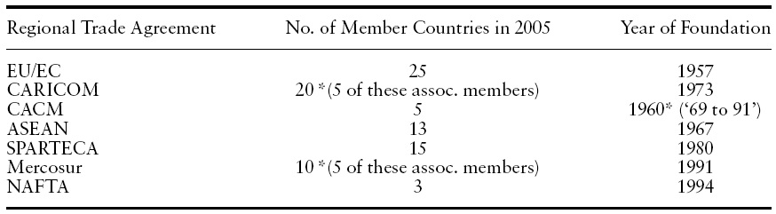
Information on the presence of a regional trade agreement, WTO membership and the currency union membership are from Andrew Rose’s Dataset. Since regional trade agreement membership may change over time, updates were obtained from the trade agreements’ websites and from the WTO websites and are summarized in Table 2.
The novel data contribution of our paper is the STE classifications. Table 3 outlines the countries in this study that use STE importers and/or exporters. These data have been assembled from an extensive analysis of the literature and from WTO notification-of-STE forms. The information on STE importers was obtained from McCorriston and McLaren (2001) on the use of STEs in Agriculture and from Abbott and Young’s (1999) paper on STE importers. As part of the WTO regulation on STEs, member countries must notify the WTO on their use of STEs. Much of the information obtained from previous research was checked against the WTO notification archives (GATT Digital Library, 2006). The bulk of the information on STE exporters was obtained from McCorriston and McLaren (2001) and notification documentation at the WTO (WTO Notifications, 2006).
[Table 2.] Regional trade agreement memberships

Regional trade agreement memberships
[Table 3.] Changes in the use of wheat STEs from 1970 to 2005

Changes in the use of wheat STEs from 1970 to 2005
Our panel data set consists of 94,716 observations of trades between trading pairs, including 19,453 non-zero trades. To provide some background for our estimations, and for comparability with the previous literature (Rose, 2004), we estimate a pooled OLS (POLS) model for a log-linearized version of the model, using only non-zero trades. Given that we have a panel dataset where unobserved effects are common, and following the recommendations of Subramanian and Wei (2003), we test and find for the presence of FE for country pairs. We thus estimate both a basic regression and fixed effects (FE) model to illustrate the robustness of our results.
As already noted, there are two significant challenges for the standard OLS estimation of log-linear gravity trade equations. First, OLS estimation of the loglinear specification does not permit the use of almost80%of the zero observations and thus is likely to suffer from serious selection bias. Considerable information is also lost in omitting the zero trades.8 Silva and Tenreyro (2006) show that standard corrections for this selectivity bias, like the Heckman two-step procedure (Heckman, 1979), are inadequate. Second, they also show that heteroskedasticity is a significant problem in the log-linear model because it creates biased estimates even when including trading-partner fixed effects.
Estimation techniques that directly permit zero values for the dependent variable include various count-data procedures, such as the Poisson PseudoMaximum Likelihood (PPML) approach.Thus,we follow Silva and Tenreyro (2006) and estimate a PPML model with FEs as our base model (using STATA software). For consistency with much of the past literature, we also estimate the PPML model without FEs. PPML estimation assumes the variance of the dependent variable is proportional to its mean.9 This is likely less binding where the number of zero trades is in the minority, such as Silva and Tenreyro’s (2006) use of aggregated trade data that include
Another problem is that our sample is more skewed using one commodity whose export market is dominated by a smaller number of countries. Hence, the assumption that the mean equals the variance as assumed in the Poisson distribution is more problematic than in more aggregated trade settings. There are twoways of handling over-dispersion (Hilbe, 2007; Cameron&Trivedi, 2010). The first is to ‘correct’ the regression standard errors for heteroskedasticity using robust procedures,which is Silva andTenreyro’s approach.Thus, all of our models employ robust standard errors that cluster upon each trading pair. The second way is to employ a Negative Binomial Regression (NBR) approach to deal with over-dispersion, which we also estimate to assess the robustness of our Poisson distribution results.
5We acknowledge that wheat is not perfectly homogeneous, as would be the ideal case of the proverbial ‘widget’.Nevertheless, it ismuchmorehomogeneous than most ‘manufactured goods’ for example, and has provided the classic example of a perfectly homogeneous product to generations of principles of economics students.. 6In a log-linearized specification, the zero-trade flows may also be dealt with using a two step Heckman procedure where the probability of a positive trade flow is first estimated using instrumental variables to construct the Inverse Mills Ratio (IMR) (Heckman, 1979). If a bias due to the omitted zero trade flows is indicated, the IMR is included in the second step to correct for the bias in which the sample is restricted to non-zero trades. A drawback with this approach is finding valid instruments. Even where this challenge is overcome, a heteroskedasticity problem remains (Silva&Tenreyro, 2006). 7Observations were deleted where: trade volume observations <1MT (1000 kg); trade value observations ≤0; constant dollar unit price range of 20
We present four different sets of results starting with (1) the Pooled OLS (POLS) using a log-linear specification that forms the comparison point with most of the literature; (2) or we show that the POLS specification is inappropriate and then estimate thePPMLmodel; (3) or, considering that almost 80% of the observations have zero trade, we estimate a zero-inflated PPML model; finally (4) showing that we have significant over-dispersion, we then estimate a NBR model (all using robust approaches). For the first two approaches,we estimate the model both with and without import country and export country STE variables of key interest to account for the role of trading partner heterogeneity. The final two approaches only report results with STE variables for brevity purposes.Overall, our empirical methodologies approximate best-practice estimation of gravity models.
5.1 Pooled OLS and Fixed Effects
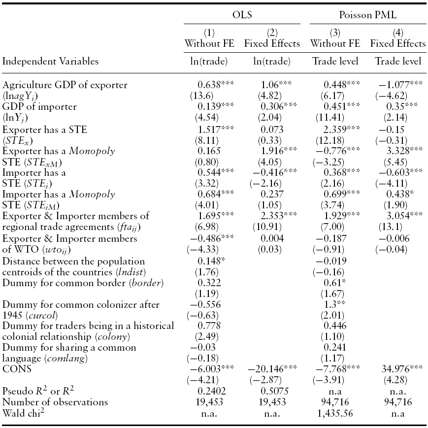
The log-linear POLS model results are presented in column 1 of Table 4, while the trading-partner fixed effects (FE) model results are reported in column 2. In general, the results in columns 1 and 3 are consistent with previous gravity trade model findings for the standard variables.The basic demand and supply variables, GDP of the importer and agriculture GDP of the exporter are both positive and significant. Most of the binary control variables performas expected, although as described below, the STE variables have unexpected results in column 1. However, as described above, if there are omitted factors about each trading partner, then the basic OLS results in column (1) are biased.
The trading partner FE POLS coefficients in column (2) should be interpreted to reflect the response to departures from the mean values for the characteristics describing each country-pair. Specifically, in the FE estimation, the identifying information for the STE coefficient comes from any change in STE status during the sample period. Thus, the FE model provides a very strong test of the effects of a STE with all other time-invariant country pair characteristics captured by the FEs. Thus, if the STE variable coefficients are significant, this suggests an impact of trade flows as the result of a change in status from having to not having an STE, or measuring the effects of beginning or removing monopoly status, which means the identification strategy is akin to natural experiment approaches.
The FE POLS coefficients in column (2) for the key STE variables are considerably different than in the POLS results in column (1).While the basic POLS results in column (1) suggest that an exporting STE alone has a positive and significant relationship with exports, the FE POLS results in column (2) suggest no statistical influence on exports. Conversely, for the FE POLS results, an exporting STE with monopoly status has a positive and statistically significant association with wheat exports of that country, while this variable is statistically insignificant in the basic POLS model. In the case of importing STEs alone, their presence is associated with reduced wheat imports in the FE POLS model, although having monopoly import status does not have any further statistical effect. These findings are again nearly the opposite of the basic POLS model in column (1). The implication is that the FE POLS results are more consistent with expectations and they illustrate that not controlling for fixed effects could lead to unexpected results.
[Table 4.] Real value of wheat trade between country pairs, OLS and Poisson models, 1970?2005
Real value of wheat trade between country pairs, OLS and Poisson models, 1970?2005
In terms of the trade institution variables, membership in a regional free trade area is positively associated with wheat trade, whereas WTO membership has no statistical impact in the FE POLS result. The latter finding is similar to that reported by Rose (2004) who found, using a POLS approach, that WTO membership did not necessarily increase the level of trade between two countries.
The log-linear POLS models are statistically inconsistent when the very restrictive conditions about the variance are unmet.To test the adequacy of the log-linear POLS specification’s assumption about the variance, we perform the Park test as described by Manning and Mulahy (2001) and Silva and Tenreyro (2006). The null hypothesis is that the variance meets the restrictions of the log-linear specification. However, the null hypothesis is rejected with a
5.2 Poisson Pseudo Maximum Likelihood (PPML)
The PPML model estimates are presented in columns 3 and 4 of Table 4. The FE PPML model in column 4 is the base model, whereas the basic PPML model without FEs in column 3 is presented for comparison. The first apparent result is that the general pattern of the STE results is similar to the corresponding POLS results – i.e. when comparing columns 1 to 3 and columns 2 to 4. Our base results are the FE PPML results in column 4. They show that the presence of an export STE alone is statistically insignificant. However the presence of a monopoly STE does have a significant and positive association with a country’s wheat exports. In the case of exporter STEs, the magnitude of the STE monopoly coefficient significantly exceeds that of the (negative) STE alone, 3.328 and −0.15 respectively. The net effect of a monopoly export STE would thus be 3.178 – the positive effect of the STE monopoly more than offsets the negative effect of the STE alone.
The presence of an import STE is negatively associated with its own imports (significant at the 1% level), suggesting that countries may use import STEs in a protectionist manner for the benefit of domestic producers. We show a negative effect of −0.603, a trade inhibiting effect that is mostly offset where the import STE has a monopoly (0.438), significant only at the 10% level, leaving a small negative net effect of −0.165.
To further assess the magnitudes of the STE effects, we utilize the STATA ‘margins’ post-estimation command. We identify the STE variables as binary variables to generate the expected trade value of the implementation of an STE, and specifically a monopoly STE between trading countries to generate the impact of the binary STE variables changing from 0 to 1. In a policy context, this will provide an indication of the importance of the debate regarding STE monopolies in international trade arenas like the WTO negotiations. The expected average marginal impact on the value of wheat exports to a trading partner, as a result of implementing a monopoly export STE, is $111 million 1990US. This must be reduced by the expected (negative) marginal effect of an export STE (without monopoly status) of –$0.893 million, leaving an average net positive impact of $110.1 million of wheat trade attributable to the implementation of monopoly export STE. To put this in context for a major STE monopoly, Canada’s top 10% of wheat trades, accounting for 86% of its total exports, had a mean value of $209 million 1990US. The marginal value of $110 million thus represents an increase in wheat exports of more than 50% attributable to the monopoly export STE. When considering Canada’s maximum exports of $2 billion (to the United States), this would represent about a 5%increase.We discuss below the results in the zero-inflated models, which produce smaller impact estimates.
Generating marginal expected impacts of import STEs as for the export STEs, we find that the implementation of an import STE reduces a country’s average imports from a trading partner by $3.8 million 1990US. If the import STE has a monopoly, this negative impact is largely offset as the average expected trade value with a monopoly import STE is $2.6 million 1990US greater than without a monopoly. The net impact of the implementation of a monopoly import STE on average wheat imports is thus –$1.2 million 1990US (−3.8+2.6). Japan, a large importer ofwheat with a monopoly import STE, serves as an example country for assessing the impact. Its average annual imports from the top 10% of its trading partners over the 2001–2005 periodwas $149 million 1990US, representing74%of all its imports. The $1.2 million reduction in imports attributable to the presence of a monopoly import STE represents 0.8% of imports from this set of trading partners, a much smaller impact than that noted for export STEs.
Bear in mind in interpreting these coefficients that most observations are zero and most of the positive-valuewheat trades are relatively modest in size. Nonetheless, these results suggest that monopoly status, not the presence of an STE, is the key factor in affecting trade patterns. Indeed, this helps explain the focus on monopoly export STE status in the current round of negotiations in the WTO.
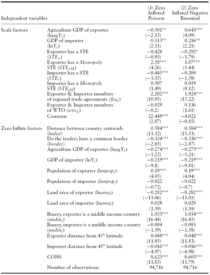
5.3 Zero-inflated Poisson and Negative Binomial Regression Models
The PPML assumes that there is not an excessive number of zero observations and that the mean and the variance of the dependent variable are equal (not over-dispersed). However, as already indicated, both of these are unlikely to hold in our particular case. First, the Gauss–Newton regression (GNR) test for the adequacy of the PPML (Silva & Tenreyro, 2006) produced a
Second, nearly 80% of the dependent variable observations are zero. Wheat trade between two countries may be zero because of the agronomic conditions or distances. Countries concentrated in the northern or the southern extremes, or on the equator are not likely to grow wheat and therefore will not be exporters. Similarly countries with large wheat producing neighbours are unlikely to be importing wheat from a more distant county as it would be more costly. Neither a standard PPML model nor a standard negative binomial regression (NBR) would allow for the observed excessive zero trades. We thus estimate a zero-inflated Poisson model (ZIP) and a zero-inflated NBR (ZINB) to assess the robustness of the base PPML results. The Vuong test for the zero-inflated versus standard Poisson yields a
Zero-inflated models are estimated in two stages: (1) a logit model to predict the probability of zero trades and then (2) a count model for positive trade values taking into account the correction for the zeros from the first stage (Hilbe, 2007; Cameron&Trivedi, 2010). In the first stage, as already described, we expect zero trades to be driven by distance and agronomic conditions, as well as production and purchasing power. These factors are shown in the bottom portion of Table 5.
The ZIP results are reported in column 1 of Table 5. The coefficients of the inflate factors (bottom half of the table) are interpreted as factors associated with producing a zero trade. The variables that appear as both scale and inflate factors will have opposite signs because their role as a scale factor indicates their contribution to larger trade values, while their contribution in the inflate factors model will indicate their contribution to effecting a zero trade. For example, GDP of the importer has positive significant coefficients as a scale factor and negative significant coefficients as an inflate factor. In addition, close proximity to 45° latitude is a strong indicator of conditions conducive to growing wheat. Thus, the positive sign of distance from 45° latitude for the exporter indicates that the farther away from 45° the country is located, the more likely that it will have zero exports. The reverse is indicated for the probability of importing.
For the scale variables of interest in the top portion of column 1 in Table 5, the presence of an export STE has no statistically significant relationship with the value of exports, while the presence of an exporting STE with a monopoly has a positive and significant effect, although the coefficient is a little smaller than in the FE PPML model in column 4 of Table 4. As in the FE PPML model, the import STE alone has a negative and statistically significant relationship, while the monopoly import STE has a positive coefficient, but it is no longer statistically significant in the ZIP (
Column (2) of Table 5 reports a zero-inflated FENBR(ZINB) regression to take into account both the over-dispersion and the excess zero values.The ZINB results further confirm a positive and statistically significant influence of a monopoly export STE, together with a (smaller) negative influence of an export STE alone (that is significant at the 10% level). This suggests that the positive monopoly influence is partly offset by the presence of an export STE alone.
The magnitudes of the impacts of implementing a monopoly STE in the ZINB are assessed as for the PPML model, using the STATA margins command. The expected average marginal impact on the value of exports to a trading partner, as a result of implementing a monopoly export STE, is $15.4 million 1990US. This must be reduced by the expected (negative) marginal effect of an export STE (without monopoly status) of –$1.1 million, leaving an average net positive impact of $14.3 million of wheat trade attributable to the use of monopoly export STE forwheat. It should be noted that this is about 1/8th of the value suggested by the PPML model above and seems more realistic. The comparable net marginal impact on average exports indicated by the ZIP was $30.7 million 1990US, closer to the ZINB regression than the PPML result. Comparing this again to actual wheat trades, Canada’s top 10% of wheat trades, accounting for 86% of its total exports, had a mean value of $209 million 1990US. The marginal value of $14.3 thus represents an average increase in wheat exports to a trading partner of about 7%associated with the implementation of a monopoly export STE. In the context of an approximate value of $2 billion 1990US to Canada’s largest trading partner, this represents about 0.7%.

Real value of wheat trade (levels) between country pairs, zero-inflated Poisson and negative binomial regression models, 1970?2005
Generating marginal expected impacts of import STEs for the ZINB model, we find that the implementation of an import STE reduces a country’s average imports from trading partners by $0.8 million 1990US. If the import STE has a monopoly, this negative impact is slightly offset as the average expected trade value with an import STE is $0.071 million 1990US greater than without a monopoly. The average net impact of the implementation of a monopoly import STE on wheat imports is thus –$0.73 million 1990US (−0.8+0.07). Again, in the context of Japan, a large importer with a monopoly import STE, this impact represents 0.5% of the average trade (2001–2005) value of $149 million, a relatively small detriment to imports.
To summarize the findings of the robustness checks, the FE POLS model, the base FE PPML model (FE), the ZIP, and the ZINB models all indicate a positive significant influence of monopoly export STEs, suggesting that the results are robust to a wide variety of specifications. That is, exporting countries with monopoly STEs appear to gain an advantage in advancing their wheat export trade with other countries. The marginal effects suggested a much larger impact for the PPML model. Given the strong evidence of over-dispersion and a zeroinflated distribution, the ZINB results are strongly preferred. Even so, the results consistently suggest that monopoly STEs benefit the export country.10 Overall, the coefficients for the scale factors, and marginal effects, in the zero-inflated models, are somewhat smaller than in the PPML, suggesting that the future studies of trade institutions should consider the problems of zero-inflation and over-dispersion in their particular setting if they use count-data methods.
The OLS FE, the base FE PPML, and the ZIP all indicate a significantly negative trade-inhibiting effect of import STEs. This is consistent with the common contention that import STEs protect domestic producers. However, both in absolute terms and as a percentage, the import STE impacts are very small.
10Further sensitivity analysis conducted for sub-samples of countries suggested the positive monopoly exporter effectwas strongestwhen the importing nationwas high income; the monopoly effect was somewhat reduced where the exporter was high income.
Contentions that STEs distort trade, both in bilateral disputes as well as at the WTO, have been longstanding and maintained largely in the absence of rigorous empirical corroboration. Domestically, STEs are often fiercely defended as serving domestic producers/consumers while at the same time proponents challenge the trade distorting allegations. However, assessments of STEs based on comprehensive empirical estimation and using current econometric techniques for policy impacts have been largely absent.
Using the WTO definition of STEs and data on 35 years of country-pair trades of wheat with a comprehensive set of control variables, this paper fills this void by conducting a quantitative analysis of the role of STEs across all countries (rather than special cases as in the past literature). Using Rose’s (2004) investigation of the role of WTO membership as a point of departure, we specify a country-pairspecific gravity trade model for wheat, including the presence of import or export STEs, as well as their monopoly status. Because omitted trading-partner fixed effects may mask the underlying relationship, we use fixed effects specifications to discern the nature of these effects. The trading-partner fixed effects account for a host of factors including institutional, transportation, slight variations inwheat varieties, or consumer preferences, which if omitted, would likely bias the results. Methodologically, this represents a more exhaustive empirical test of the role of STEs than has been available to date and our paper represents a methodological extension for using count data to assess trade in gravity models.
Based on shortcomings of the log-linear gravity equation, both in terms of dealing with heteroskedasticity, and the exclusion of zero-trade observations, we use a fixed-effects Poisson pseudo-maximum likelihood model as our base model. We find that a monopoly export STE enhances the exporting country’s value of wheat shipments. Importer STEs generally have a negative effect on the value of wheat imports, although this effect is relatively small and not further affected by monopoly status of the STE. Sensitivity analysis with zero-inflated Poisson and negative binomial regressions further confirmed the export STE results, though import STE resultswere insignificant in the negative binomial models. Our examination of zero-inflation problems and over-dispersion represents an extension of the work by Silva and Tenreyro (2006).
The implications of our results may be inferred both in terms of international trade distortions and domestic policy. The increased wheat exports associated with monopoly export STEs and the negative effects of import STEs may be indicative of trade distortion. In particular, given that wheat is typically thought to be more homogeneous than most manufactured products, this finding for wheat STEs would suggest even stronger STE findings in cases where there is more product differentiation. In WTO negotiations, these are critical issues, but until now this point was based more on assertions than on empirical evidence across all international wheat trades. Fromthe point of view of domestic policies, the apparent evidence of possible trade distorting effects and the consequences for trade agreements and other trade frictions must be weighed against the country’s commitments to domestic lobbies that benefit from STEs.