As the international integration of goods, services and assets markets has proceeded, linkages among economies in terms of prices, interest rates and exchange rates have been broadly studied. Many recent studies on international integration in the Pacific Basin have concentrated on linkages between the region’s developing economies versus Japan and the US. According to the results of these studies, there appears substantial increasing integration of domestic and international goods and financial markets. For instance, Glick and Hutchison (1990) find that the degree of linkage between domestic real interest rates in Pacific Basin countries and those in the US increased as financial liberalization in the region proceeded. Kim (1998) reveals that the degree of international capital mobility has increased rapidly in Korea since the 1980s. Ji and Kim (2009) examine the linkage of real interest rates of a group of Pacific Basin countries from 1980 to 2006 and find that the degree of capital market integration has rapidly increased since the Asian Financial Crisis of 1997-1998. In light of recent advances in market integration in the Asia-Pacific region, this article makes an empirical investigation of long-run and short-run economic linkages between Korea and the US, using a cointegrated vector autoregressive (VAR) methodology developed for the analysis of nonstationary time series data. This introductory section, as a background study, gives a review of the Korean economy as well as the related literature, then moves on to the account of our contributions to the research field of Asia-Pacific economic relationships.

When the Korean economy grew rapidly during the 1960s and 1970s, the financial sector was treated as a means of allocating available financial resources to the priority sectors, in particular, export sectors. Financial liberalization policies were adopted in the early 1980s, when the government launched a comprehensive program of economic liberalization and opening. While traderelated finance and foreign direct investment had already been mostly liberalized, flows of both portfolio investment and short-term capital were gradually liberalized. Thus, during the 1980s, the government occasionally controlled the international capital flows, considering the balance of payments, exchange rate and monetary management.

The Korean won was pegged to the US dollar until March 1980, when the government switched to a multicurrency basket peg (MCBP) system. The exchange rate was determined as a weighted average of the SDR basket and Korea’s own basket of currencies, with the government influencing the exchange rate. In February 1990, the MCBP system was replaced by a market average rate (MAR) system. The “market average rate” of the won against the US dollar was calculated by taking a weighted average of exchange rates. The market average rate became the basic rate of the following business day, and the exchange rate was allowed to fluctuate within a certain band around the basic rate. As Jwa (1994) points out, concern over possible exchange rate appreciation, especially during the late 1980s, turned out to be one of the main impediments to the liberalization of capital flows, but with the introduction of the MAR system, a more conducive environment was created for capital flow liberalization. The government eventually adopted a flexible exchange rate system in December 1997, at the onset of the financial crisis.

Until 1980, interest rates were strictly controlled by the authorities in Korea. The government started to deregulate interest rates from the early 1980s as inflationary expectations became low due to successful stabilization policies. The call rate (money market rate) was liberalized in 1984. The favorable situation in the form of price stability, high growth, and current account improvement in the late 1980s led the Korean government to continue financial liberalization. National savings exceeded domestic investment, which resulted in narrowing interest differentials between regulated rates and free market rates. In the early 1990s, the government further deregulated interest rates. By 1993, interest rates on the borrowing and lending of financial institutions were almost completely deregulated.

Let us turn to a real interest rate parity hypothesis, which is seen as one of our primary empirical interests and referred to as a real interest parity condition in this paper. Early studies using a classic regression analysis showed that the condition did not empirically hold; see, for example, Cumby and Obstfeld (1984), Mark (1985) and Cumby and Mishkin (1986). More recent studies utilizing the cointegration methodology obtained more favorable, but still mixed evidence on the real interest parity. Frankel (1992) decomposes the real interest differential into the country premium (which is the covered interest differential) and the currency premium (which is the sum of exchange risk premium and expected real depreciation). He shows that mainly the currency premium leads to the failure of the real interest parity. Kugler and Neusser (1993) investigate monthly ex post real interest rates from several countries, and find that real interest rates are mostly stationary. Considering transaction costs that include brokerage costs, information-gathering costs and implicit risk costs, Goodwin and Greenes (1994) support the real interest parity for developed countries. Jorian (1996) investigates the validity of real interest parity across the US, the UK and Germany, and indicates that there is no tendency for expected real interest rates to be equalized.

For Asian developing economies, several studies lead to mixed evidence on the real interest parity between some Asian countries and Japan and/or the US. Chinn and Frankel (1995) investigate the relative influence of the US and Japanese real interest rates in the determination of local Pacific Rim real interest rates. Korea appears to be more closely linked with Japan than with the US. The real interest parity holds for only the real interest rate pairs of US-Singapore, US-Taiwan and Japan-Taiwan—and neither US-Korea nor Japan-Korea. Hahm (1997) finds that the exact version of the real interest parity is rejected in Korea. Phylaktis (1997) shows that, in a group of Pacific Basin countries, there was an increase in capital market integration with both the US and Japan during the 1980s. In particular, the interest differential of Korea over the period 1981-1993 appeared to be stationary. Phylaktis (1999) demonstrates that the interest differential of Korea over the period of 1972-1993 was cointegrated with that of either Japan or the US. Holmes and Maghrebi (2004) test the real interest differentials of four developing Asian economies, including Korea, with respect to Japan and the US. In the case of Korea, the stationarity of real interest differentials with respect to Japan and the US is shown.

In regard to the purchasing power parity or the stationarity of the real exchange rate, there is a lot of research on the won-dollar exchange rate, whose results are mixed. Park (1995) demonstrates that the PPP hypothesis does not hold for the won-dollar exchange rate. Choi (1997) shows that the real won-dollar exchange rate follows a random walk. Chou and Shih (1997) reveal that the Johansen test supports the long-run purchasing power parity for Hong Kong and Singapore and that a fractional cointegration arises in the case of Korea. Kim (1998) indicates that the PPP hypothesis does not hold for the won-dollar exchange rate.

As the real exchange rate often appears to be non-stationary, the existing cointegration studies in international finance tend to focus on linkages between the real exchange rate and macroeconomic fundamentals such as inflation and interest rates. Some studies have not been favorable of such linkages, while others have shown evidence for stable linkages. Meese and Rogoff (1988) find little evidence of a stable relationship between real interest rate differentials and real exchange rates in Germany, Japan, the UK and the US. Thus, they suggest that real disturbances (such as productivity shocks) may be a major source of exchange rate volatility. Edison and Pauls (1993) show that real exchange rates and real interest rates are not cointegrated with each other. Cheng (1999) examines the relationships between exchange rates, relative prices, and interest rates for Japan and the US. Causality running from the interest rate to the exchange rate is found in the short run, while causality running from the price ratio to the exchange rate via the interest rate is found in the long run. MacDonald and Nagayasu (1998) find two cointegrating vectors on the domestic price and the exchange rate from a set of the yen–dollar exchange rate, home and foreign prices, and home and foreign interest rates. Juselius and MacDonald (2004) show that key parity conditions between the US and Japan did not hold as stationary relations, which, they suggest, arises from the non-stationarity of the real exchange rate. Kurita (2007) investigates theory-consistent cointegrating relationships between the real yen-dollar rate, interest rate differentials and other economic fundamentals. The current account balance in Japan appears to play an important role in determining the real exchange rate along with the interest rates. In regard to Korea, there are several studies. Kim (1995) shows that the won-dollar exchange rate has a stable long run relationship with the current account balance and interest rate differentials. Lee (1997) and Lee and Choi (1998) incorporate several macroeconomic variables to explain and/or forecast the won-dollar exchange rate. Kim and Kwon (2003) successfully apply the real interest differential theory of Frankel (1979) to the Korean won exchange rate determination.

The review of the Korean economy and literature given above, overall, leads to a motivation for the empirical exploration in this article. It seems that the literature on the real interest parity, exchange rate determination and current account equation is separated in most cases, although all of these three themes are deeply related to important international financial aspects of the economies in question.1 The results of previous studies, as explained above, show mixed evidence on real interest parity. In addition, one should bear in mind the fact that there were restrictions to capital flow in Korea. In light of these issues, we introduce in our study a loose-form real interest parity condition, combined with possible long-run economic linkages centering on the real exchange rate and current account. It turns out, as demonstrated in a series of sections below, that our study indicates that Korea and the US have been closely associated with each other through interest and foreign exchange rate channels. To the best of our knowledge, this article seems to be the first empirical study that has succeeded in revealing a picture of the two countries’ close linkages through these financial channels. The overall empirical results are, therefore, expected to be informative for both policy makers and macroeconomists who take interest in the Asia-Pacific economy.

The rest of this article is organized as follows. Section II reviews a cointegrated VAR model and economic implications of cointegrating vectors, and Section III then provides a canonical model on a loose-form real interest parity, real exchange rate behavior and current account. Section IV presents an overview of the data, and Section V performs a cointegrated VAR analysis of the data in order to reveal long-run economic relationships. Section VI estimates a parsimonious vector equilibrium correction system so as to investigate the underlying short-run dynamics. The overall summary and conclusion are given in Section VII. All the numerical analyses and graphics in this article use OxMetrics / PcGive (Doornik and Hendry, 2007).

1Exceptional works using the cointegrated VAR methodology are, among others, Kurita (2007) on exchange rates and the current account in Japan, and Choo and Kurita (2011) on monetary interaction aspects in Korea.

This section briefly reviews the likelihood-based analysis of a cointegrated VAR model for time series data of integrated of order 1, denoted by I(1) hereafter. The VAR model is introduced by Johansen (1988) and is explained by Johansen (1996) and Juselius (2006). Let us consider a cointegrated VAR(k) model for a p-dimensional time series, X_–k+1,...,X_T, which is given by

where D_t is an s-dimensional vector of deterministic terms apart from the intercept, such as seasonal and impulse dummies, and the innovations є_t,..., є_T have independent and identical normal N(0,Ω) distributions conditional on the initial values X_–k+1,...,X_T. The parameters in Equation (1) vary freely and are defined as α, β ∈ R^p×r, γ∈R^r for r˂p, Г_i, Ω∈R^p×p, and Ω is positive definite. Let us define β^*’=(β’,γ) and X^*_t–1=(X’_t–1,1)’ for future reference. A set of vectors α is called adjustment vectors, while β* is referred to as cointegrating vectors.

The cointegrating rank r in Equation (1) is, however, usually unknown to investigators; thus the rank needs to be determined from the data analysis. A log-likelihood ratio (logLR) test statistic is given by the null hypothesis of r cointegration rank H(r) against the alternative hypothesis H(p) and is denoted as logLR(H(r)|H(p)). Its asymptotic quantiles are provided by Johansen (1996, Ch.15). See also Nielsen (1997) and Doornik (1998) for the method of gamma approximations to calculate the quantiles. Determining the cointegrating rank allows us to test various restrictions on α and β*. Cointe- grating relationships, embodied by β*’X^*_t–1 correspond to a set of I(0) linear combinations, and they act as equilibrium correction mechanisms in Equation (1). Thus, the relationships can represent long-run economic linkages of variables in the system. It is therefore important to check if theory-consistent restrictions can be imposed on β*, as estimated from the data.

This section introduces a canonical economic model, which is subject to the study of long-run economic relationships using Equation (1). We consider two countries: home and foreign. The ex ante relative purchasing power parity (PPP) and uncovered interest parity (UIP), respectively, are given as follows:

where p_t is the natural logarithm of price level, s_t is the natural logarithm of a spot exchange rate defined as the domestic price of foreign currency, and i_t is the nominal interest rate. The superscripts e and * denote expected values and foreign variables, respectively. Substituting Equation (2) into Equation (3) yields:

Equation (4) is called the real interest parity. Let ppp_t = p_t – p^*_t – s_t denote the natural logarithm of real exchange rate,2 and

denote an expected change in the real exchange rate. The failure of (deviation from) the ex ante PPP given by Equation (2) implies that Δppp^e_t+1 is different from zero. Following Cumby and Obstfeld (1984), we may incorporate Δppp^e_t+1 into Equation (4), allowing for the failure of the ex ante PPP given by Equation (2). Thus we obtain

We may also incorporate a risk premium into Equation (3), and thus into Equations (4) and (5) as well, allowing for the failure of (deviation from) the UIP given by Equation (3). Adjusting for such possible failure of the PPP and UIP in a real-life economy, we may consider that Equation (5) leads to a candidate for an empirical loose-form real interest parity. Since the expected inflation rate is never observed, we may invoke rational expectations, so that the expected inflation rate equals the actual inflation rate plus a forecast error whose mean is zero. Then Equation (5) may correspond to a cointegrating relationship estimated from the data, provided that the expected change in the real exchange rate (Δppp^e_t+1), the risk premium, and forecast errors are all approximated as stationary processes. In other words, we may find

where a constant term cons. takes account of the unobserved components, which may be stationary variables with non-zero means. Note two points: (i) we have allowed for the failures of (deviations from) the PPP and UIP and (ii) we have assumed the stationarities of expected change in the real exchange rate, the risk premium, and forecast errors. The first point is needed to incorporate restrictions on capital flows in Korea, which were explained in Section I. The second point is somewhat strict, which needs to be verified, but is just assumed here to make the analysis simple. Expression (6) means that the linear combination of the variables is seen as an I(0) process as a whole, thus corresponding to a long-run cointegrating relationship. We shall refer to this relationship as Equation (6) like other equations, although this is not an equation in the exact sense of the word.

Let us then turn to a set of equations for the real exchange rate and the current account balance, which is denoted by ca_t. First, let us assume that the expectation formation for depreciation of the nominal exchange rate is explicitly given by

where u_t denotes an I(0) error term, and the parameter δ satisfies 0 ˂ δ ˂ 1 such that the exchange rate expectation gradually adjusts to disequilibrium errors from the PPP level, that is, p_t – p^*_t – s_t. Equation (7) may thus be referred to as a PPP-based expectation formation. Moreover, let Equation (3) be explicitly modified by adding a time-varying risk premium ϕ_t to it as follows: 3

Suppose that ϕ_t is empirically represented by ca_t, so that we can replace ϕ_t with ca_t in Equation (8).4 Thus, combining Equations (7) and (8), we can then find

where θ=1/δ so that θ is greater than 1 due to the restriction 0 ˂ δ ˂ 1. We are justified in claiming that the approximation given by Equation (9) is compatible with that of Equation (6) as long as the maturities of interest-bearing bonds differ. Equation (6), for example, may be defined in terms of long-term interest rates, while short-term interest rates may appear in Equation (9) instead. This is because differences in maturities can lead to discrepancies in the time series properties of the underlying risk premiums, thereby generating the possibility that both approximations, Equations (6) and (9), can empirically hold as paired cointegrating relationships. As mentioned in Section I, Kim (1995) shows that the won-dollar exchange rate has a stable long-run relationship with the current account balance and interest rate differential, as in Equation (9). For instance, during the late 1980s when the exchange rate was partly controlled by the authorities, the Korean won was subject to strong appreciation pressures because of the current account improvement and favorable interest rate differential. In addition, we may also find the following relationship is empirically relevant to our study:

where ω is a non-negative parameter for the real exchange rate. Equation (10) implies that the current account balance tends to be affected by real exchange rate behavior through international price competitiveness. Kim (2001) shows that in Korea in the 1990s, capital inflows (which could be affected by the interest differential) caused the real exchange rate to appreciate, as shown by Equation (9), and that the real exchange rate appreciation led to the current account deficits, as shown by Equation (10). Chang (2009) demonstrates that the real exchange rate is the most effective determinant of the Korean trade balance, as in Equation (10).

This section gives an overview of the time series data in Korea (the home country) and the US (the foreign country), running from the first quarter in 1981 to the first quarter in 2010 (denoted 1981.1-2010.1 hereafter). The overview helps us to explore the possibility that such long-run economic linkages as shown in Equations (6), (9) and (10) in the previous section, may empirically hold in the data for the two countries. A subsequent formal analysis of long-run relationships is performed in the next section. See Appendix A for details on the data.

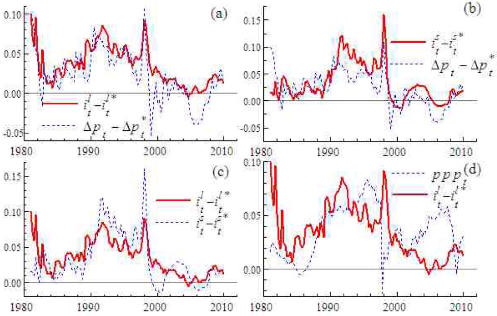
Figure 1(a) presents a long-term interest rate differential (i^l_t – i^l_t*) and an inflation differential (Δp_t – Δp_t*) between Korea and the US. The similarity in trending behavior suggests the presence of a cointegrating relationship between the two series, coinciding with the loose-form real interest parity given by Equation (6). Note that several spikes are witnessed in the data around the end of the 1990s. They correspond to the Asian currency crisis, which gave rise to large-scale devaluations of a number of Asian currencies. Figure 1(b) provides a short-term interest rate differential (i^s_t – i^s_t*) and Δp_t – Δp_t*. The behavior of i^s_t – i^s_t* does not look so close to that of Δp_t – Δp_t*, as compared with Figure 1(a). In Figure 1(c), long-lasting deviations are found in between i^l_t – i^l_t* and i^s_t – i^s_t*, indicating their weak linkage.

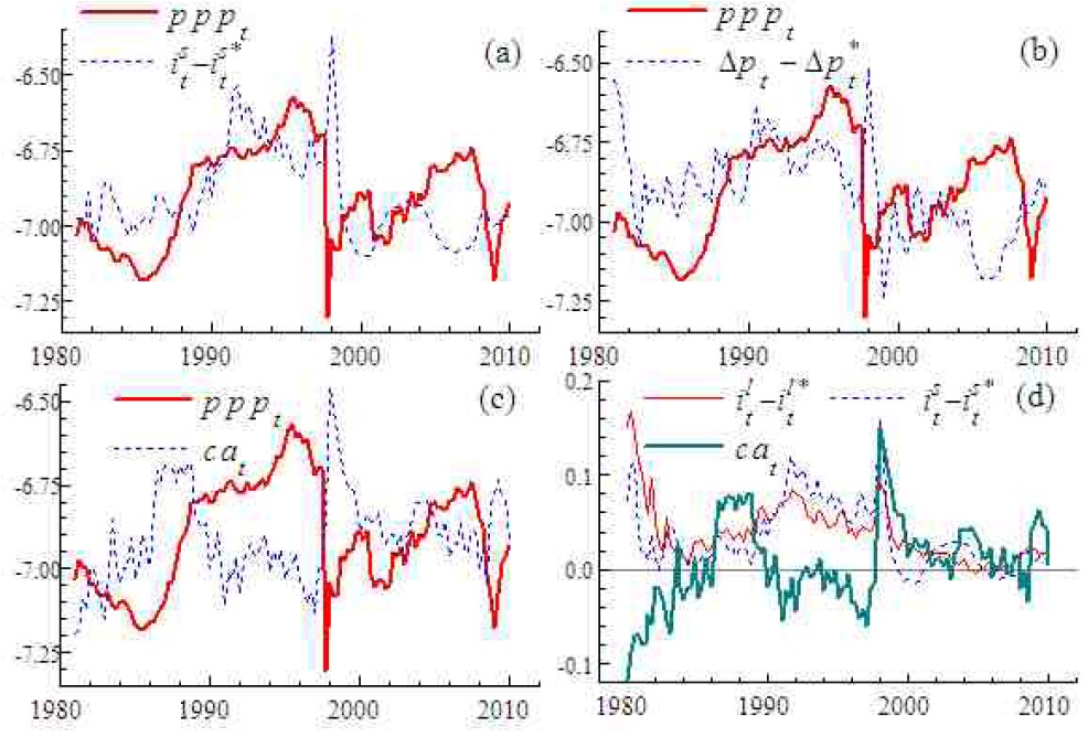
Figure 1(d) presents the real won-dollar rate (ppp_t) and i^l_t – i^l_t*, with the scale of the figure given along the vertical axis being normalized for i^l_t – i^l_t*. In addition, ppp_t, i^s_t – i^s_t* and Δp_t – Δp_t* are provided in Figures 2(a) and (b), whose scales are both normalized for ppp_t. These figures indicate that ppp_t appears to be more closely related to i^s_t – i^s_t* than i^l_t – i^l_t* and Δp_t – Δp_t* although the linkage between ppp_t and i^s_t – i^s_t* may be so weak that we cannot find a cointegrating relationship as it stands. Some combinations of these two variables with other variables, however, may lead to such an interpretable cointegrating relationship as is developed in Section III. Figure 2(c), normalized for ppp_t, shows the ratio of a current account balance to nominal GDP in Korea (ca_t). Both ppp_t and ca_t seem to exhibit countercyclical behavior to some degree, which corresponds to the equation for current account (10). Figure 2(d) displays ca_t, i^l_t – i^l_t* and i^s_t – i^s_t*. A countercyclical feature appears to be present in between i^s_t – i^s_t* and ca_t, apart from the period for the currency crisis. Thus both Figures 2(a) and (d) suggest that ppp_t, if combined with such variables as i^s_t – i^s_t* and ca_t, may also lead to an interpretable cointegrating relationship like Equation (9).

2Note that a rise in pppt denotes a real appreciation of the Korean won.  3Note that when the risk premium ϕt is high, the domestic interest rate it is low and/or the foreign interest rate i*t is high, according to the definition on the risk premium ϕt in Equation (8).  4That is, we suppose that an improvement in the current account cat of the home economy is positively related to either a rise in the risk premium of the foreign economy, ϕt, or a fall in the risk premium of the home economy, –ϕt.

Motivated by the arguments in Sections III and IV, we select the set of variables to be analyzed as follows:

which leads to a five-dimensional VAR system formulated as Equation (1). Other variables like income, wealth and depreciation rate are not explicitly taken into account here, as they can be empirically irrelevant in the context of a cointegration analysis.

The sample period for estimation is 1981.1-2010.1, thus the number of observations available for estimation is 117. The lag length of the VAR model is set at 3 based on F-test statistics for the model reduction. The VAR model also includes centered seasonal dummy variables. It turns out, however, that the estimated model suffers from autocorrelation and autoregressive conditional heteroskedasticity (ARCH) effects in the residuals. As shown by Equation (1), the VAR model is formulated in such a way that a set of dummy variables can be incorporated in order to render the estimated innovations reasonably-well distributed. It is, therefore, justifiable to include in the model batteries of dummy variables for large-scale outliers, as long as they are attributable to economic and social incidents recorded in history. We thus introduce the following blip and impulse dummy variables, all of which correspond to historical events:

and zero otherwise. D_m,t captures several outliers caused by changes in the US monetary policy stance (see OECD, 1983). D_ca,t mitigates an outlier in 1997.1, possibly caused by two factors: (i) the Korean current account deficit resulting from a deterioration in the terms of trade and (ii) increased uncertainty in the Korean economy due to labor strikes opposing a policy change towards more flexible labor markets. D_ca,t also allows for Korea’s current account deterioration in 1999.1 in the aftermath of the financial crisis. D_ppp1,t corresponds to the Asian currency crisis in 1997.4. During the crisis, the Korean government was forced to request financial support from the IMF, and then pursued such policies as abiding by the IMF’s recommendations. D_ppp2,t picks up an outlier in 2000.4, possibly reflecting increased uncertainty in the Korean market due to the implementation of corporate and financial restructuring plans. Finally, D_ppp3,t captures an outlier corresponding to the global financial crisis in 2008.3. Influences of these dummy variables on inference are inspected in the auxiliary cointegration analysis in Sub-section 3 below.

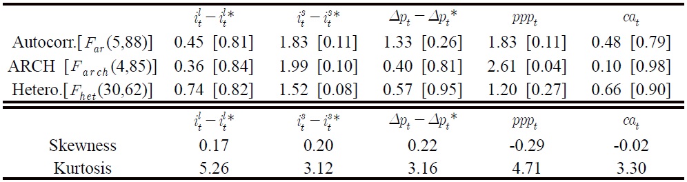
Table 1 presents a set of diagnostic tests on the residuals of the unrestricted VAR model. The first panel reports the test results in the form F_j(k, T–l), which denotes an approximate F-test against the alternative hypothesis j: kth-order serial correlation (F_ar: see Godfrey, 1978, Nielsen, 2007), kth-order ARCH (F_arch), and heteroskedasticity (F_het: see White, 1980). Most of these three test statistics do not reject the null hypotheses at the 5% level, indicating that the model’s residuals do not suffer seriously from temporal dependence and heteroskedasticity. According to the second panel, however, kurtosis statistics for the residuals from i^l_t – i^l_t* and ppp_t equations are much larger than 3, suggesting a rejection of the normality assumption. The overall skewness statistics, relatively speaking, seem to be less problematic than kurtosis. Simulation studies such as Cheung and Lai (1993) and Gonzalo (1994), show that Johansen’s procedure for cointegration analysis is sensitive to residual autocorrelation, while it is robust to excess kurtosis. The absence of residual autocorrelation, ARCH and heteroskedasticity may allow us to conclude that the unrestricted VAR model can be subject to the subsequent multivariate cointegration analysis, at the cost of some efficiency loss stemming from non-normal residuals.

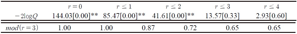
Table 2 presents the logLR test statistics for cointegrating rank, in addition to the modulus of the six largest roots of a companion matrix for the model.

The logLR test statistics for the cointegrating rank, denoted as –2logQ in the first panel, sequentially reject the null hypotheses of r = 0, r ≤ 1 and r ≤ 2, hence supporting r = 3. The second panel provides a modulus (denoted mod) of the six largest eigenvalues of the companion matrix restricted with r = 3. All the eigenvalues, apart from the first and second ones, appear to be distinct from the unit root, and there is no evidence for an explosive root. Moreover, using a procedure suggested by Johansen (1996, p.74), we have also tested to see if each variable is individually stationary or not. The hypothesis of stationarity is rejected with respect to each variable in the VAR system at the 5% significance level. The overall evidence, thus, allows us to reach the conclusion that the model is expressible as an I(1) cointegrated VAR model with the number of the cointegrating vectors given by r = 3.

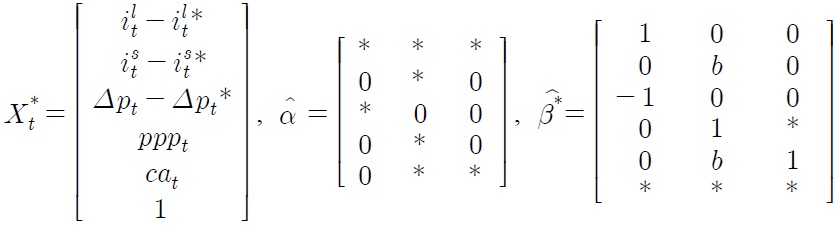
A series of trials, motivated by the discussion in Section III and the data overview in Section IV, have led to a set of acceptable joint restrictions as follows:

Asterisks in

matrices denote coefficients on which no restriction is imposed, while b indicates a coefficient on which a homogeneity restriction is imposed. Note that the three cointegrating relationships are normalized for i^l_t – i^l_t*, ppp_t and ca_t, respectively. The restricted estimates

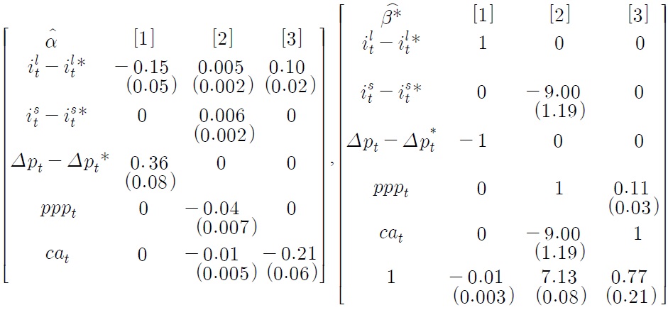
, most of which are rounded to the second decimal place, are reported in Table 3, together with the corresponding logLR test statistic. The p-value of the test statistic is 0.19, so the null hypothesis for the joint restrictions is not rejected at the 5% level. Significant coefficients are given in Table 3, together with the corresponding standard errors in parentheses.

The restricted cointegrating relationships in the table are denoted by c_1,t, c_2,t and c_3,t, respectively. The first relationship is

which corresponds to the loose-form real interest parity given by Equation (6). It is noteworthy that such a simple linear combination of i^l_t – i^l_t* and Δp_t– Δp_t*, augmented with a constant term, leads to an I(0) cointegrating relationship. The value of the constant term is –0.01, i.e. –1% which can be interpreted to reflect an expected real appreciation, risk premium and/or forecast error. According to the left panel of Table 3, the adjustment coefficients for i^l_t – i^l_t* and Δp_t– Δp_t* are highly significant, while the remaining coefficients are all insignificant and therefore set to zero. As demonstrated by Johansen (1996, Ch.3), cointegrating relationships act as attractor sets or equilibrium correction mechanisms in a cointegrated VAR system. Thus, we find that an equilibrium correction mechanism embodied by c_1,t is only at work for i^l_t – i^l_t* and Δp_t– Δp_t*, rather than for the remaining variables. This finding indicates a close and stable linkage between i^l_t – i^l_t* and Δp_t – Δp_t*, supporting the validity of the empirical loose-form real interest parity.

The second cointegrating relationship is, according to Table 3, given by

which coincides with Equation (9), thus being interpreted as the modified UIP condition [see Equation (8)] combined with the PPP-based expectation formation [see Equation (7)]. Note that the parameter θ is estimated to be 9.00, implying that the estimated parameter for expectation adjustments in Equation (7) is approximately 0.11 or

This estimate indicates that expectation adjustments towards the PPP level occur gradually, which seems to agree with our intuition. As c_2,t is an identified cointegrating relationship normalized for ppp_t, it is possible to consider that ca_t and i^s_t – i^s_t* share common stochastic trends with ppp_t, thereby accounting for the long-run behavior of ppp_t. In fact, ppp_t reacts to this second cointegrating relationship in a highly significant way, as shown in the left panel of Table 3. Thus, c_2,t may be treated as evidence for the existence of a stable linkage between the real exchange rate and various economic fundamentals.

Finally, the third relationship is

which is interpreted as a current account equation given by Equation (10). The interpretation is based on the conjecture that a rise in ppp_t leads to a reduction in Korea’s price competitiveness, thereby decreasing exports and increasing imports. The adjustment coefficient for ca_t is highly significant and thus shows the presence of steady equilibrium correction. The adjustment coefficient for i^l_t – i^l_t* is also significant, indicating some spill-over effects of the equilibrium correction on i^l_t – i^l_t*. Note that i^l_t – i^l_t* reacts to all the disequilibrium errors represented by the three cointegrating relationships. In light of the overall evidence reported in Table 3, the long-term interest rate differential seems to play a key role in the economic integration of Korea and the US.

In addition, as a complementary comparative study, the same analysis as above is conducted using the VAR model excluding all the blip and impulse dummy variables, with the result that batteries of fairly similar coefficients are obtained. See Appendix B for a table recording these coefficients. Overall, the similarity between the estimates for the two VAR models seems to support the validity of the adjustment and cointegrating structure reported in this section. As a caveat, let us recall that it is not justifiable to try to make reliable inferences solely based on this auxiliary VAR model, whose estimated innovations are much affected by large-scale outliers triggered by various historical events. See Sub-section 1 for details.

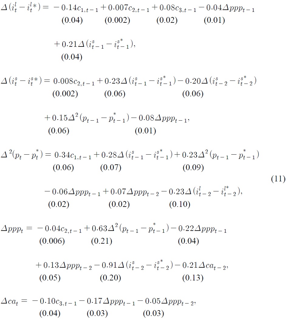
We are now in a position to estimate a parsimonious vector equilibrium correction system based on the cointegration analysis above. Removing insignificant regressors from the model step by step, we have arrived at a parsimonious system as follows:

where the figures in the parentheses are standard errors and all the dummy variables are omitted for the sake of simplicity in exposition. The adjustment structure of the parsimonious system is in accord with that found in Table 3.

According to system (11), Δppp_t–1 plays a significant role in accounting for the short-run dynamics of all the equations and all the coefficients for the Δppp_t–1 terms hold negative values. With regard to the equations for Δ(i^l_t – i^l_t*) and Δ(i^s_t – i^s_t*), the negative coefficients of Δppp_t–1 may be understood in such a way that the appreciation of the real won-dollar rate has a downward impact on the competitiveness of the Korean economy, thereby leading to reductions in domestic interest rates. The appreciation of the real won-dollar rate should, at the same time, have a deflationary effect on prices in Korea. Both Δppp_t–1 and Δppp_t–2 hold almost the same value with an opposite sign in the equation for Δ²(p_t–p_t^*), indicating that the acceleration of the real appreciation of the won-dollar rate, or Δ²ppp_t–1, has indeed a deflationary impact on Δ²(p_t–p_t^*). In regards to the Δppp_t equation, the negative coefficient of Δppp_t–1 may represent volatile behavior of the real won-dollar rates, i.e. its appreciation leads to depreciation in the subsequent quarter and vice versa. In the equation for Δca_t, the negative coefficients of Δppp_t–1 and Δppp_t–2 seem to reflect a decrease in price competitiveness, which has a downward impact on Korea’s trade balance.

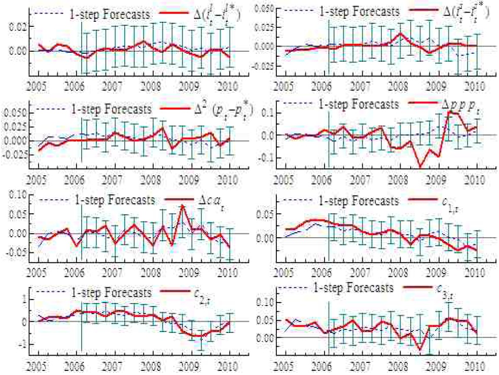
Finally, Figure 3 displays sequences of 1-step forecasts of Δ(i^l_t – i^l_t*), Δ(i^s_t – i^s_t*), Δ²(p_t–p_t^*), Δppp_t, Δca_t, c_1,t, c_2,t and c_3,t, together with their 95% confidence bands. The forecast horizon consists of 16 observations, so the estimation sample is truncated to 2006.1. According to the figure, there seems to be no evidence for systematic or persistent forecast failures, although a large impact from the global financial crisis in 2008 is observed in the forecasts of Δppp_t, Δca_t and c_3,t. Figure 3 suggests that the system was subject to the global financial crisis, but free from any structural factors causing a series of persistent mis-forecasts.

This paper shows that the estimated cointegrated VAR system, which consists of interest rate differentials, the real won-dollar rate and several macroeconomic variables of Korea and the US, encompasses three long-run relationships interpretable from economic theory. The first relationship agrees with a loose-form real interest parity condition, the second is consistent with a real exchange rate equation and the third is viewed as a current account equation. A parsimonious vector equilibrium correction system is subsequently estimated so that the structure of the underlying short-run dynamics can be inspected. Lastly, the study demonstrates that the preferred parsimonious system is informative as a macroeconomic forecasting device. Overall, the study supports the view that the two economies have been closely associated with each other through interest and foreign exchange rate channels. The results presented in this article are, as a whole, seen as useful empirical information for policy makers as well as macroeconomists who are interested in the underlying interdependent relationships in the Asia-Pacific region.