This paper investigates the relationship between the trade balance, foreign income, money supply, real exchange rate, and domestic income of South Korea’s economy. This inquiry is worthwhile because if exchange rate depreciation does not improve the trade balance, stabilization packages that include some exchange rate realignment cannot be justified. It is important for policymakers to understand whether changes in real exchange rates can be used as a policy tool to manipulate trade flows.
This study differs from the extant literature in at least two dimensions. First, we focus exclusively on South Korea because of its important trade and economic characteristics. South Korea is Asia’s fourth-largest economy and the world’s 12th-largest economy measured by purchasing power parity. South Korea is a member of the United Nations, WTO, OECD, and G-20 economies and a founding member of APEC and the East Asia Summit. South Korea is an Asian Tiger and to date the only developed country included in the Next Eleven countries. The South Korean economy is export-driven and heavily dependent on international trade. In 2010, South Korea was the world’s sixthlargest exporter and 10th-largest importer. However, few studies examine the relationship between trade balance and its determinants in South Korea.
Second, we have adopted three fully efficient estimation methods: fully modified OLS (FMOLS) (Phillips and Hansen, 1990), canonical cointegrating regression (CCR) (Park, 1992), and dynamic OLS (DOLS) (Saikkonen, 1992; Stock and Watson, 1993). The FMOLS procedure involves the use of Wald tests, where the resulting test statistics are “fully modified” by semi-parametric corrections for serial correlation and for endogeneity. This fully modified procedure has been found to work well in finite samples. The CCR procedure also removes the long-run dependence between the cointegrating equation and stochastic regressors’ innovations. In addition, the key advantage of the DOLS procedure is that it allows for the presence of a mix of I(0) and I(1) variables in the cointegrated system. DOLS corrects for potential endogeneity problems and small sample bias and provides estimates of the cointegrating vector that are asymptotically efficient.
We organize the rest of the paper as follows. In the next sections, we present a theoretical background of the Keynsian view, J-curve, and Marshall-Lerner condition. Section III provides a brief overview of selected literature. Section IV provides a theoretical framework. Section V discusses the data and reports results. Section VI concludes and offers policy recommendations.
Ⅱ. Marshall-Lerner Condition, J-Curve and the Keynsian View
Given that an individual country is small relative to the rest of the world, one condition that is required for a successful depreciation is the fulfillment of the Marshall-Lerner condition, i.e., sum of import and export demand elasticities exceeding unity. However, the Marshall-Lerner condition is considered a long-run condition. The J-Curve concept, which was introduced in 1973 by Magee (1973), asserts that it is possible for depreciation to worsen the trade balance in the short-run before showing improvement.
According to the Keynesian approach, exchange rate depreciation affects the relative prices of domestic goods in domestic currency. This reduction produces two forms of direct effects. First, there is an income effect, which would increase absorption, and then reduce the trade balance. Second, there is a substitution effect that causes a shift in the composition of demand from foreign goods to domestic goods that is the exchange rate change causes an expenditure-substituting effect.
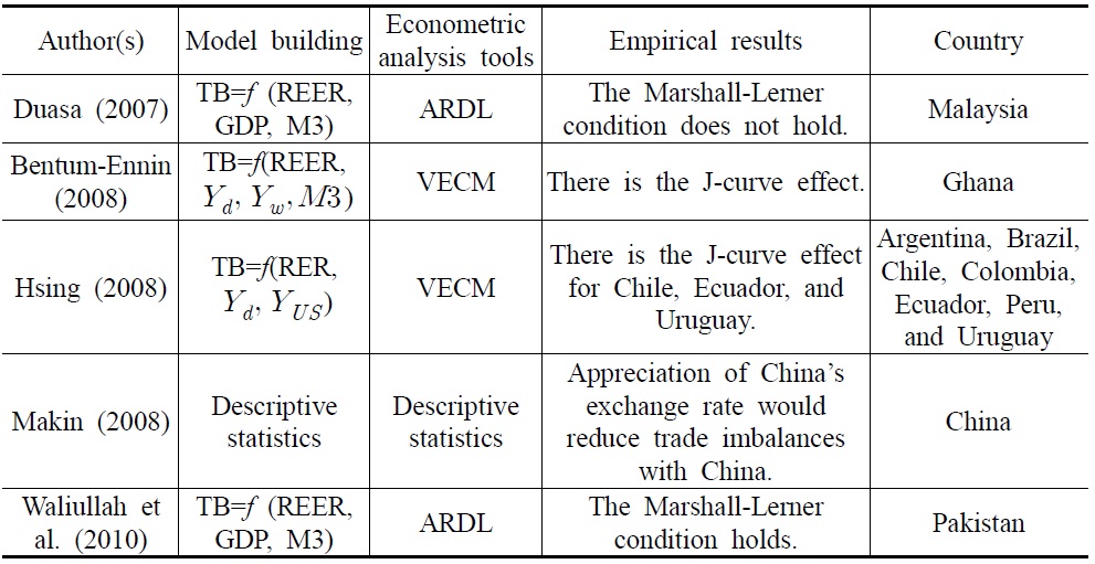
Despite popular belief that depreciation can improve the trade balance, the empirical studies tend to suggest mixed results (See Table 1). For example, Duasa (2007) examines the relationships between trade balance, real exchange rates, income, and money supply in Malaysia. Using an autoregressive distributed lag (ARDL) approach to cointegration, those variables are found to be cointegrated, and the study suggests that the Marshall-Lerner condition does not hold in the long-run for Malaysia. Duasa (2007) adds that the Malaysian trade balance or balance of payments should be viewed from absorption and monetary approaches. However, Duasa’s (2007) study is not a sufficient work on the specification of trade balance. It is worth noting that the foreign income is ignored by Duasa (2007) without further clarification. It may raise a question about the biases of omitting other relevant variables in modeling trade balance behavior.
[Table 1] Comparison of Previous Literature

Comparison of Previous Literature
Bentum-Ennin (2008) analyzes the responsiveness of the balance of trade to changes in real exchange rates. He examines the time pattern of this response to verify the existence of the J-curve phenomenon in Ghana. He finds that the real exchange rate has a positive long-run relationship with Ghana’s trade balance, demonstrating that depreciation leads to an improvement in the trade balance.
Hsing (2008) finds evidence of a J-curve for Chile, Ecuador, and Uruguay and a lack of support for a J-curve for Argentina, Brazil, Colombia, and Peru. An increase in real income in the home country would improve trade balances for Brazil and Ecuador and worsen trade balances for Argentina, Chile, Colombia, Peru, and Uruguay. An increase in real income in the U.S. would improve the trade balance for Argentina, Chile, Colombia, Peru, and Uruguay and worsen trade balances for Brazil and Ecuador.
Makin (2008) evaluates China’s exchange rate policy and current account surplus in the context of its rapid development under the hypothesis that undervaluation of the Yuan against major currencies is central to any explanation of global imbalances. He argues that the currency misalignment has resulted in China’s industrialized trading partners, notably the U.S. and the European Union, simultaneously experiencing larger bilateral current account deficits with China, lower output, lower saving, and higher investment. He suggests that significant appreciation in China’s exchange rate would simultaneously reduce China’s huge trade surplus and the bilateral deficits of its trading partners.
Recently, Waliullah et al. (2010) examine the short-run and long-run relationships between the trade balance, income, money supply, and real exchange rate in Pakistan’s economy. Their results provide persuasive evidence that money supply and income are prominent in determining the behavior of the trade balance. The exchange rate regime can help improve the trade balance, but will have a weaker influence than growth and monetary policy.
Surprising, there is no existing literature on South Korea’s trade balance. Also, there is no previous paper using cointegrating regression methods as econometric analysis tools. To the best of our knowledge, this paper is the first to investigate the determinants of South Korea’s trade balance using cointegrating regression methods.
Our model begins with the assumption that the quantity of imported goods demanded depends on the domestic income and the relative price of imported goods:

where

where
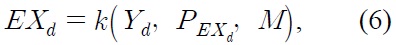
The quantities of goods available for export depend on the relative price of exports and on the level of production:


where
A monetary variable, M, is included in the import demand and export supply functions. The extended import demand and export supply functions are as follows:

In the following equilibrium conditions, we can determine quantities and prices:


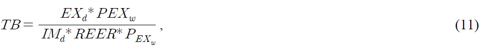
The value of the domestic trade balance is as follows:

where
Model 1 has the form:

Model 2 has the form:

Here, TB is trade balance, M1 is the narrow money supply, M3 is the broad money supply, IP is a measure of domestic income, WORLD is a measure of foreign income, REER is a measure of the real effective exchange rate, is an error term, and
1In order to allow for a currency substitution between South Korea and the rest of the world, we used a measure of the real effective exchange rate. The traditional IMF measure of the real effective exchange rate uses a weighted average of foreign prices, with weights reflecting the home country’s bilateral trade with each foreign country. The advantage of this definition is that it enables a comparison of domestic and international prices over time.
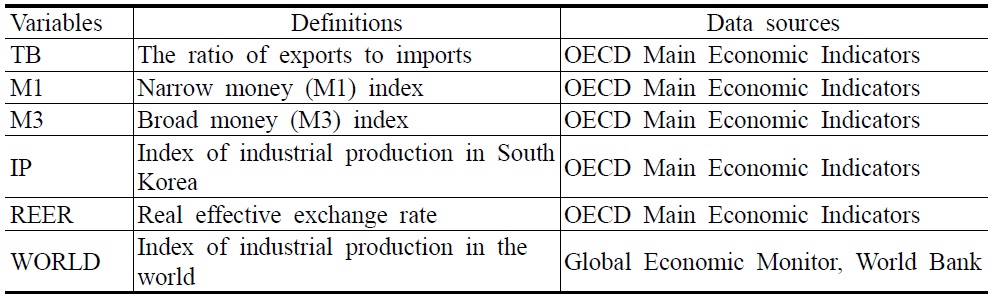
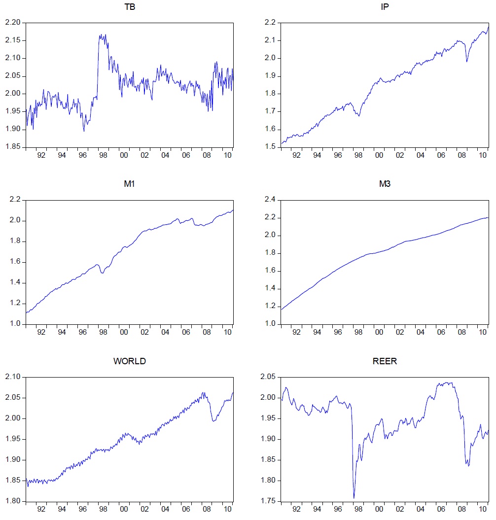
Table 2 contains descriptions and sources of the variables used in this research. Data used for the empirical exercise are monthly for the period of January 1991–January 2011 and are obtained from the OECD Main Economic Indicators. In the Appendix, we provide complete details on the different variables. All variables are seasonal adjustments of the data. To reduce heteroscedasticity, all variables are transformed into natural logarithms. Time series plots of the variables are presented in Figure 1.
[Table 2] Definitions of Variables and Data Sources

Definitions of Variables and Data Sources
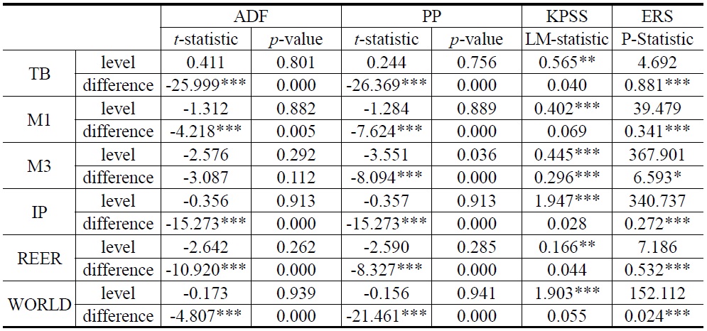
Properties of the variables must be investigated in order to avoid the possibility of spurious regressions. We use augmented Dickey and Fuller (1979, ADF), Phillips and Perron (1988, PP), Kwiatkowski-Phillips-Schmidt-Shin (1992, KPSS), and Elliott-Rothenberg-Stock point optimal (ERS, 1996) unit root tests. All unit root tests (except KPSS) in our study have a null hypothesis that the series in question has a unit root against the alternative of stationarity. In contrast, the null of KPSS states that the variable displays stationarity. Results of the unit root tests are presented in Table 3 and, in most cases, seem to indicate that all variables are integrated of order 1, that is, I(1).
Unit Root Tests
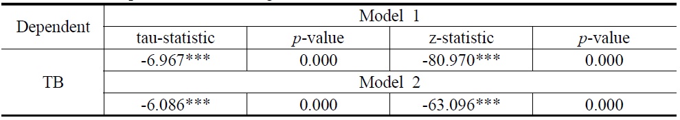
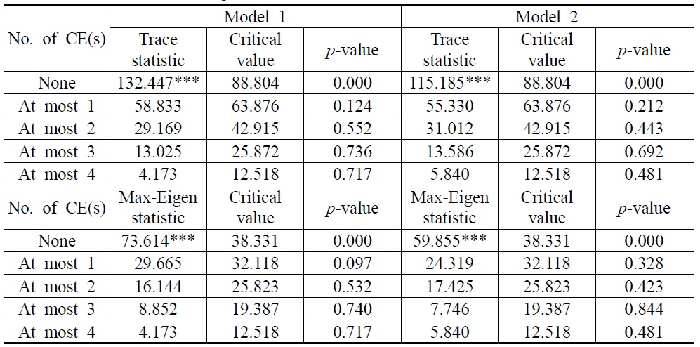
To test for a long-run relationship among the variables, we apply the Johansen (1988) cointegration tests, the residual-based tests of Engle and Granger (1987) and Phillips and Ouliaris (1990), and Park’s added variables test (Park, 1992). Results from the Johansen cointegration tests are presented in Table 4. Both the maximum eigenvalue and the trace statistics indicate there is one cointegration vector in Model 1 and Model 2. On the other hand, the cointegration results tabulated by Engle and Granger, and the Phillips and Ouliaris residual-based tests are in Tables 5 and 6. For both Models 1 and 2, we reject the null hypothesis of no cointegration.
[Table 4] Johansen Cointegration Test
Johansen Cointegration Test
[Table 5] Engle and Granger Cointegration Test

Engle and Granger Cointegration Test
[Table 6] Phillips-Ouliaris Cointegration Test

Phillips-Ouliaris Cointegration Test
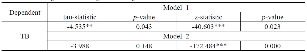
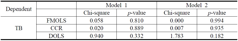
Finally, the results of Park’s added variables test are reported in Table 7. Park (1992) outlines a test of the null hypothesis of cointegration against the alternative of no cointegration. We find that the Chi-square test statistics do not reject the null hypothesis of no cointegration. Hence, trade balance, real money supply, domestic income, exchange rate, and foreign income are cointegrated.
[Table 7] Park Added Variables Cointegration Test

Park Added Variables Cointegration Test
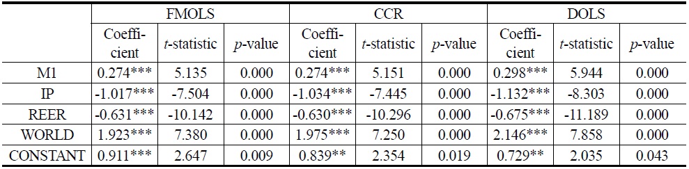
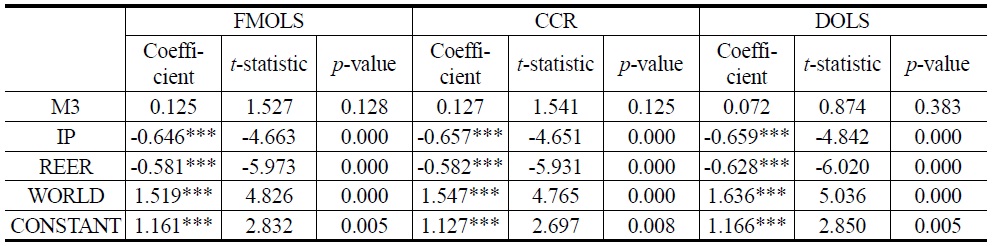
In Tables 8 and 9, results of three different estimators (FMOLS, CCR, and DOLS) are reported for Model 1 and Model 2, respectively. We find that WORLD has a statistically significant and positive impact on money demand. For example, the elasticity of WORLD ranges from 1.923 to 2.146, implying that a 1% increase in WORLD leads to, at most, a 2.146% increase in Model 1. Meanwhile, the elasticity of WORLD ranges from 1.519 to 1.636 in Model 2. Since the response is relatively elastic, South Korea’s trade balance is likely to improve from growth in foreign income.
Additionally, IP has a statistically significant and negative effect in both Models 1 and 2. For instance, a 1% increase in IP decreases TB by 1.017 to 1.132% in Model 1 and 0.646 to 0.659% in Model 2. IP is a negative sign, which is consistent with the theory. According to theory, it has a negative impact in country trade balances because an increase in our domestic level of income causes less availability of goods to export.
The impact of the REER on the trade balance is negative and statistically significant. It suggests that the Marshall-Lerner condition holds in the long-run. The depreciation of domestic currency by 1% on average improves the trade balance by 0.630-0.675% and 0.581-0.628% as suggested by Model 1 and Model 2, respectively. It indicates that the sum of elasticities of exports and imports exceeds unity in the long-run and that depreciation improves the trade balance.
[Table 8] Cointegrating Regression for Model 1

Cointegrating Regression for Model 1
[Table 9] Cointegrating Regression for Model 2

Cointegrating Regression for Model 2
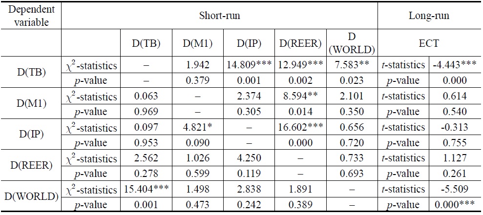
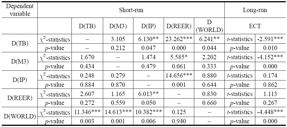
Tables 10 and 11 report the results of short-run and long-run Granger causality for Model 1 and Model 2, respectively. Beginning with the short-run results, the chi-square tests of the explanatory variables indicate the significance of the short-run causal effects. We can find a unidirectional causality from REER and WORLD to TB.
[Table 10] Granger Causality Tests for Model 1

Granger Causality Tests for Model 1
In terms of long-run results, t-statistics for coefficients of the lagged error-correction terms indicate the significance of the long-run causal effects. The coefficient of the one-period-lagged error correction term is statistically significant with a negative sign in the trade balance equation for Models 1 and 2. This result suggests that all variables Granger-cause South Korea’s TB in the long-run.
[Table 11] Granger Causality Tests for Model 2

Granger Causality Tests for Model 2
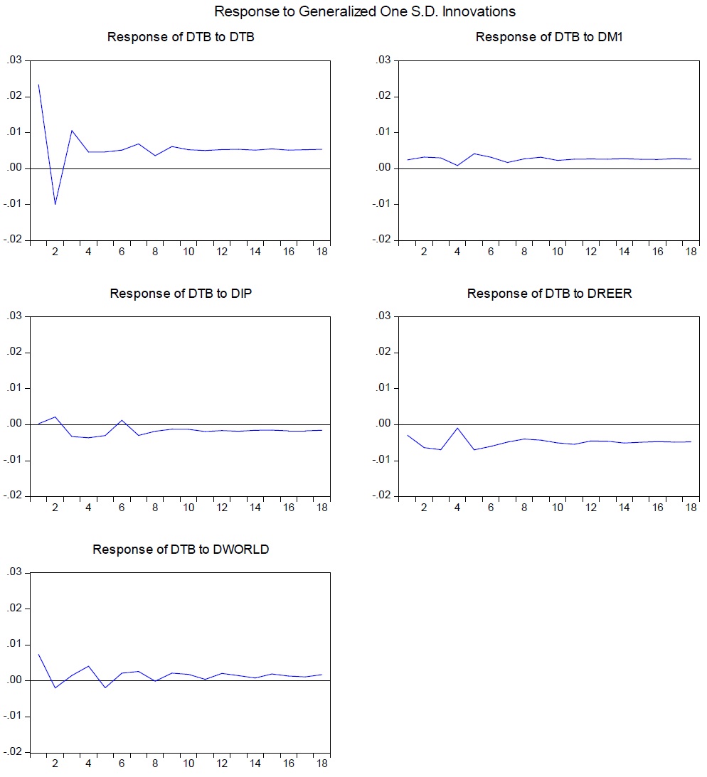
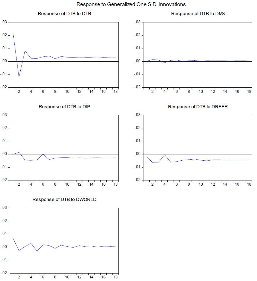
6. Generalized Impulse Response Functions
The generalized impulse response results are depicted in Figures 2 and 3. The months after the impulse shocks are shown on the horizontal axis. The vertical axis measures the magnitude of the response. An appreciation will immediately deteriorate South Korea’s trade balance for about three months, after which it briefly improves, indicating some form of the inverted J-curve effect. Subsequently, the trade balance deteriorates again and remains in deficit.
Moreover, the trade balance reacts to domestic income innovations as it responds negatively. This result conforms to the Keynesian view that a rise in domestic income encourages more demand for imported goods and therefore worsens the trade balance.
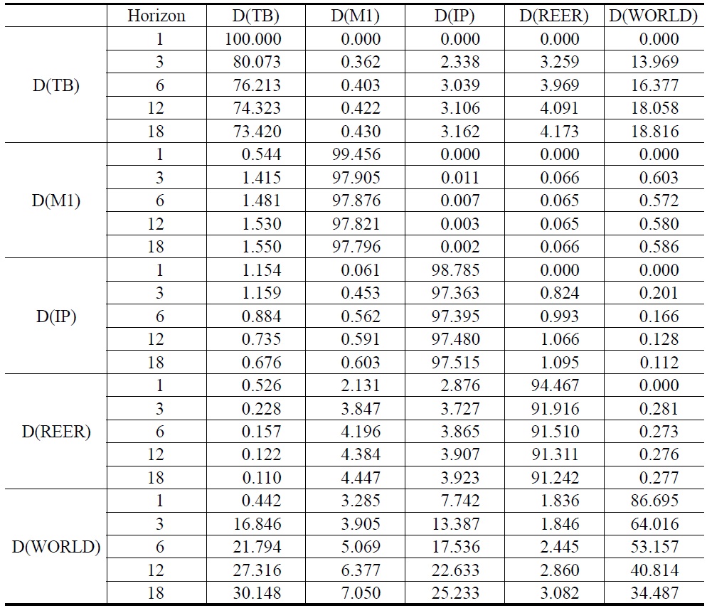
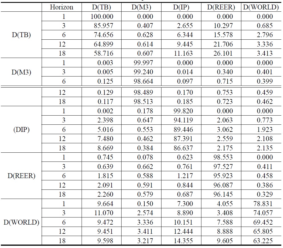
7. Forecast Error Variance Decomposition
Forecast error variance decomposition provides an optimal measure of the amount of forecast error variance decomposition for each variable that would result from a different possible ordering of the variables. Table 12 reports the results of the forecast error variance decomposition in Model 1. We find that the impact of D(WORD) can explain 18.816% of the forecast error variance of trade balance in the long-run. Results of the forecast error variance decomposition for Model 2 appear in Table 13. After 18 months, the impact of D(REER) explains 26.101% of the forecast error variance of trade balance in Model 2.
[Table 12] Forecast Error Variance Decomposition for Model 1

Forecast Error Variance Decomposition for Model 1
[Table 13] Forecast Error Variance Decomposition for Model 2

Forecast Error Variance Decomposition for Model 2
8. Comparison of Results with the Previous Literature
On the basis of the cointegration tests results, we conclude that South Korea’s trade balance and its determinants are cointegrated. Also, Duasa (2007) shows that there is a cointegration relationship among the variables using a bound testing approach for Malaysia. Consistent with our finding, Bentum-Ennin (2008) finds that there is a J-curve effect in Ghana. Moreover, our finding for the Marshall-Lerner condition is consistent with that found by Waliullah et al. (2010). However, the Marshall-Lerner condition does not hold from the work of Duasa (2007), which utilizes an ARDL approach.
Ⅵ. Conclusions and Policy Implications
This paper has examined the relationships between South Korea’s balance of trade and each of its four important determinants. The results suggest a long-run relationship between trade balance, real effective exchange rate, foreign income, money supply, and domestic income. Upon estimating the trade balance model using three different estimators (FMOLS, CCR and DOLS), it was clear that foreign income is the most important determinant of the trade balance, followed by domestic income and real effective exchange rate.
Two policy implications emerge from our analysis. First, the impact of the exchange rate on the trade balance is negative and statistically significant. This finding suggests that the Marshall-Lerner condition holds in the long-run in the case of South Korea. Appreciation of South Korea’s currency by 1% on average weakens its trade balance by 0.675% and 0.581%. This finding indicates that the sum of elasticities of exports and imports exceeds unity in the longrun. The exchange rate is a potent policy tool to realign South Korea’s balance of trade.
Finally, consistent with the Keynesian view, increases in domestic income will encourage the general public to purchase more imported goods and thus worsen South Korea’s trade balance. There is a need to search out import substations to fill the import demand and to establish policies regarding improvement in the volume of qualitative exports. Domestic supply increases and a regulatory framework to assure supply of goods are needed.