An autoregressive distributed lag (ARDL) approach to cointegration is used to examine the dynamic effects of changes in the bilateral exchange rate on changes in the bilateral exports and imports of disaggregating 71 products between Korea and the United States. Results show that while Korean exports are highly sensitive to the U.S. income and less to the bilateral exchange rate change in both the short- and long-run, Korean imports are driven largely by the income of Korea and, to some extent, by the bilateral exchange rate. It is also found that the empirical results obtained from aggregated data of trade are at odds with our findings of disaggregated data, providing partial evidence of the aggregation bias problem, as well as the importance of use of disaggregating data in bilateral trade models.
Since the collapse of the Bretton Woods system in 1973, a plethora of studies have been conducted to analyze the effect of exchange rate fluctuations (i.e., devaluation) on the trade balance in developed and developing countries. Early studies conducted in the late 1980s and the early 1990s have typically employed aggregate trade data in the framework of a two-country model (i.e., between a country and the rest of the world) in investigating the exchange rate impact on the trade balance (e.g., Bahmani-Oskooee 1986, Felmingham 1988, Mahdavi and Sohrabian 1993). In the early 2000s, empirical studies argued that, since a country’s trade balance could improve with one trading partner while simultaneously deteriorating with another, the use of aggregate data between a country and the rest of the world, instead of a bilateral level, could lead to aggregate bias of data, thereby resulting in a misinterpretation of the dynamics of the trade balance in response to exchange rate fluctuations. For this reason, the second group adopts bilateral trade data between a country and its major trading partners to tackle the issue (e.g., Wilson 2001, Arora et al. 2003, Bahmani-Oskooee and Ratha 2004).
More recent studies, however, have claimed that a country tends to export (import) different commodities to (from) different trading partners, and significant exchange rate effects with some commodities could be more than offset by an insignificant exchange rate impact with others and vice versa; hence, the empirical findings, even from the second group, also could be related to the aggregation bias of data (e.g., Bahmani-Oskooee and Ardalani 2006, Bahmani-Oskooee and Wang 2007, Bahmani-Oskooee and Bolhasani 2008). Further, the third group argues that by dealing with exports and imports as a single variable in a trade balance model, studies both in the first and second groups are not able to directly detect what variables (i.e., exchange rates) are affecting exports and/or imports and by how much, thereby providing misleading results. As a result, this new body of literature uses industry/commodity level data on a bilateral basis and, at the same time, analyzes exports and imports separately in order to accurately measure the effects of exchange rate fluctuations on the trade balance.
Until recently, however, studies in the trade literature on Korea have typically constituted the first and second groups as classified earlier (e.g., Bahmani-Oskooee and Ratha 2004, Chang 2005 and 2009, Kim 2009). Chang (2005), for example, examines the effect of the real exchange rate on the trade balance between Korea and the rest of the world, which falls into the first group. He finds that exchange rates have little effect on the trade balance. Kim (2009) analyzes Korea’s bilateral trade with the U.S. and Japan, which constitutes the second group and finds that depreciation of the U.S. dollar has a significant effect on the Korea’s trade balance. Accordingly, relatively little attention has been paid to investigate the impact of exchange rate fluctuations on Korea’s exports and imports at a bilateral industry/commodity level.
In this study, we have attempted to expand the trade literature by examining the effect of exchange rate fluctuations on Korea’s exports and imports within the context of disaggregating 71 industries’ bilateral trade data of between Korea and the United States. The empirical focus is on the characteristics of the short- and long-run dynamics and empirically identify whether Korea’s trade with the United States could benefit from a decline in the value of the U.S. dollar. Since the beginning of Korean economic development in the early 1960s, the trading relationship between Korea and the United States has been an important one. In 2009, for example, the U.S. was the third-largest trading partner for Korea (after China and Japan), and Korea was the seventh largest U.S. trading partner (after Canada, China, Mexico, Japan, Germany, and the United Kingdom).
The remainder of this paper is organized as follows. The next section introduces the empirical model associated with the ARDL estimation. The following section describes the data used for the analysis as well as the empirical procedure. The last two sections discuss the empirical results and make some concluding remarks.
1In fact, during 1965-1995, the U.S. was the largest trading partner of Korea, accounting for 20~40% of Korea’s total trade. China has overtaken the United States as Korea’s leading trading partner since 2000 (currently around 20% of total trade).
To examine the effect of exchange rate changes on exports and imports between Korea and the United States, we rely on the bilateral inpayments (export values) and outpayments (import values) models developed by Bahmani-Oskooee and Goswami (2004) and Bahmani-Oskooee and Ardalani (2006). In its simplest form, this model can be stated as follows:


where

where
It is worth mentioning that in investigating the exchange rate impacts on trade flows, studies have generally related the
For each commodity (or industry) group


where

is the real U.S. income;

is the real income of Korea; and
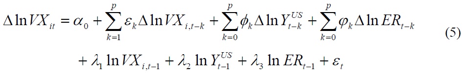
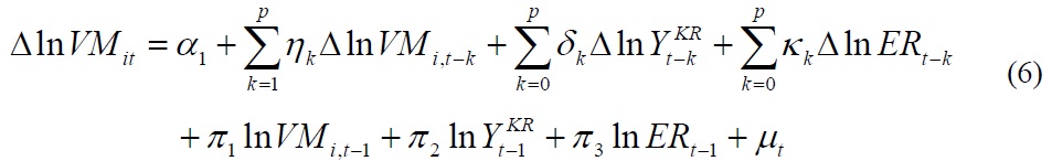
Following Pesaran et al. (2001), equations (3) and (4) are reformulated as the ARDL framework, which involves an error-correction modeling format as follows:


where Δ is the difference operator; and
2It should be admitted that the use of an aggregate price index (i.e., exchange rate), instead of an industry (sectoral)-specific price index, could also lead to aggregate bias of data. In fact, export and import price indices (at bilateral commodity level) may be available in some cases. As such, a trade volume approach could be more desirable than a trade value approach in investigating the exchange rate-trade nexus. One serious weakness of such indices, however, is the assumption that exporters charge the same prices in domestic and foreign countries for each exported commodity and/or that importers pay the same price to all exporting countries for each imported commodity. This assumption may not be valid in any real economic sense and raises the issue of specification error due mainly to an inadequate specification of data elements (Cushman 1987 and 1990). In this regard, the trade value approach is considered an alternative model specification to pursue this line of research.
Ⅲ. Data and Empirical Procedure
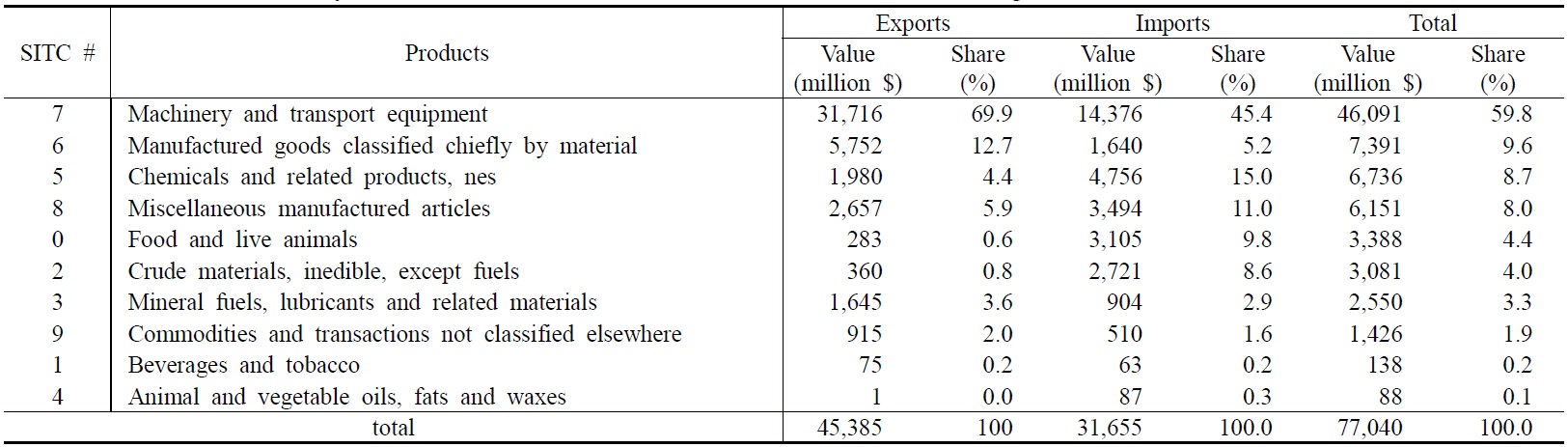
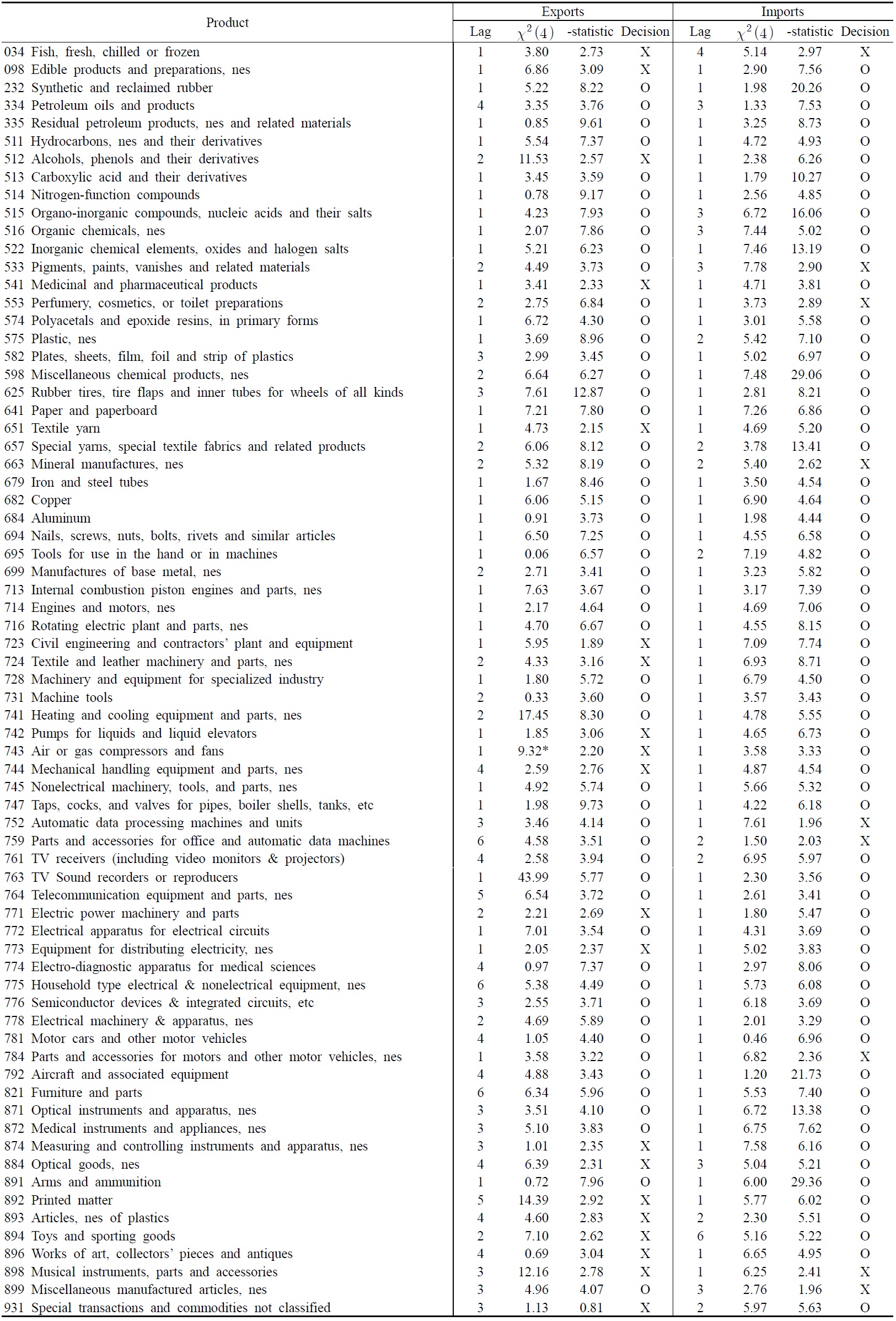
The data used for the analysis are collected between the first quarter of 1989 and the third quarter of 2009 (1989:q1-2009:q3). The values of exports and imports for industries (3-digit Standard International Trade Classification, SITC) between Korea and the United States are collected from the Interactive Tariff and Trade Dataweb in the U.S. International Trade Commission (USITC). Using the average 2005-09 trade share of each industry, we then identify the 71 most-important trade industries between the two countries (Table 2).
2. Testing Procedure for the ARDL
As the first step in applying the ARDL procedure, we determine lag lengths (
The results of the
A possible criticism of our attempts to explore the exchange rate impacts on Korea-U.S. bilateral trade is that, although the ARDL is found to perform better for small sample sizes than other cointegration methods, finite sample analysis could still bias the test toward identifying the long-run relationship either too often or too infrequently. However, as noted by Hakkio and Rush (1991), “our Monte Carlo studies show that the power of a cointegration test depends more on the span of the data rather than on the number of observations. Furthermore, increasing the number of observations (particularly by using monthly data instead of quarterly and annually) does not add any robustness to the results in tests of cointegration.” Following this study, our data used for the analysis (83 observations for the period 1989-2009) are considered to be long enough to reflect the long-run relationship among the variables; hence, this should somehow mitigate the concern with the degree of the finite sample bias of the cointegration test and does not undermine the credibility of our findings.
3It is worth mentioning that, since the trade data used for the analysis are measured from the U.S. perspective, they capture costs as paid by the U.S. Korea’s exports (U.S. imports) are calculated as CIF (cost, insurance, and freight) values in order to incorporate all costs involved up to arrival in the U.S. Korea’s imports (U.S. exports) are calculated as FOB (free on board) values to exclude all costs after shipment. As a result, Korea’s exports measured by CIF prices might reflect changes in transport costs, whereas Korea’s imports, expressed by FOB prices, might not. In addition, because of the unavailability of Korean export data in the late 1980s and/or the early 1990s, the following 11 industries have shorter time periods: (1) SITC 334 (1991:q1-2009:q3), (2) SITC 512 (1998:q2-2009:q3), (3) SITC 513 (1992:q2-2009:q3), (4) SITC 516 (1995:q3-2009:q3), (5) SITC 522 (1995:q1-2009:q3), (6) SITC 533 (1993:q2-2009:q3), (7) SITC 541 (1991:q4-2009:q3), (8) SITC 574 (1992:q2-2009:q3), (9) SITC 598 (1992:q2-2009:q3), (10) SITC 682 (1993:q3-2009:q3), and (11) SITC 684 (1992:q4-2009:q3). 4The Akaike Information (AIC) and Schwartz-Bayesian Criteria (SBC) are the two most popular model selection criteria. SBC is known as the parsimonious model – selecting the smallest possible lag lengths. On the other hand, AIC is known for choosing the maximum relevant lag lengths. In this study, the AIC is used to select the model for the following reasons: (1) Since the AIC provides the optimal maximum lags in a model, it is well suited to capture the dynamic effects of exchange rate changes on exports and imports; and (2) the mean prediction errors of AIC based models are generally lower than those of SBC based models.
With the cointegrating relationship being identified, we use the selected ARDL model outlined by equations (5) and (6) to estimate the long-run coefficients and error-correction model. The results of the long-run coefficient estimates of the Korean export function show that the exchange rate is not statistically significant in the majority of cases. Of the 51 industries in which all three variables are cointegrated, for example, 37 industries are found to be statistically insignificant even at the 10% level, accounting for approximately 73% of all industries. This indicates that, in the long-run, the bilateral exchange rate plays little role in determining Korea’s exports to the United States (Table 3). One possible explanation for this finding is that, as the value of the Korean won (U.S. dollar) increases (decreases), Korean exporters squeeze their profit margins to offset the increase in their export prices in order to maintain their share of the U.S. market, thereby having little effect on export earnings (Haynes et al. 1986, Bahmani-Oskooee and Wang 2009). Another plausible explanation for this is that, since high-technology industries are well known to confront less price competition than traditional industries in international markets, the structural changes in leading Korean export items towards high-tech and high-quality products over the past decades may have been an important factor in reducing the impact of exchange rate changes on exports (Table 1). The coefficients of the exchange rate, on the other hand, are found to be statistically significant at the 10% level for 14 industries; the average coefficient is +1.73, indicating that a 1% depreciation of KRW increases inpayments (export earnings) by 1.73%. It is important to notice that the bilateral exchange rate is indeed a significant determinant of Korea’s major export products to the U.S. for categories such as telecommunications (17.2% of total exports) and motor vehicles (19.7% of total exports) (Table 3). The real U.S. income, by contrast, is found to be statistically significant at the 5% level in all but two industries (SITC 759 and 776). Of the 49 industries in which the real U.S. income is found to be statistically significant, for example, 46 industries show a positive long-run relationship between Korean exports and real U.S. income, the average coefficient is +4.81, suggesting that a 1% increase in U.S. real income improves inpayments by 4.81%. For the remaining 3 industries (SITC 752, 763, and 899), on the other hand, Korean exports have a negative long-run relationship with the real U.S. income, implying that an increase in real income in the U.S. causes a decline in Korea’s export values.
For the Korean import function, the results of the long-run coefficient estimates show that the exchange rate is found to have statistically significant coefficients in more than half of the industries (Table 4). Of 62 industries in which all three variables are cointegrated, for example, 35 industries show a negative long-run relationship between Korean imports and bilateral exchange rate. Their average coefficient is -1.33, indicating that a 1% decrease in the value of the Korean won worsens the outpayments by 1.33%. For the remaining 27 industries, however, the exchange rate is found to be statistically insignificant even at the 10% level. This finding further suggests that import industries in Korea are more responsive to the bilateral exchange rate than export industries. Note that, unlike the export function, the bilateral exchange rate has little effect on Korea’s major import products from the U.S. such as semiconductor devices and aircraft, indicating some evidence of non-price competition (Table 4). The coefficients on the real income of Korea are statistically significant at the 10% level in the majority of cases (50 out of 62 industries), suggesting that the real domestic income is an important factor in affecting Korea’s imports from the United States (average coefficient: +1.72).
It is worth mentioning that market shocks such as the Asian Financial Crisis (DUM1; 1997:q3-1998:q4) and the recent financial crisis (DUM2; 2007:q3-2009:q3) may result in a change in Korea-U.S. trade flows over the sample period. To capture such effects, two dummy variables are included in the estimation. Of the 51 export industries (62 import industries) in which all three variables are cointegrated, for example, the estimated long-run coefficients of DUM1 and DUM2 turn out to be significant only in 14 and 16 cases (20 and 21 cases), respectively, suggesting that these market shocks have little impact on the bilateral trade.
To identify the short-run dynamics that seem to exist between Korea’s trade and its main determinants, we estimate first differenced variables in equations (5) and (6).
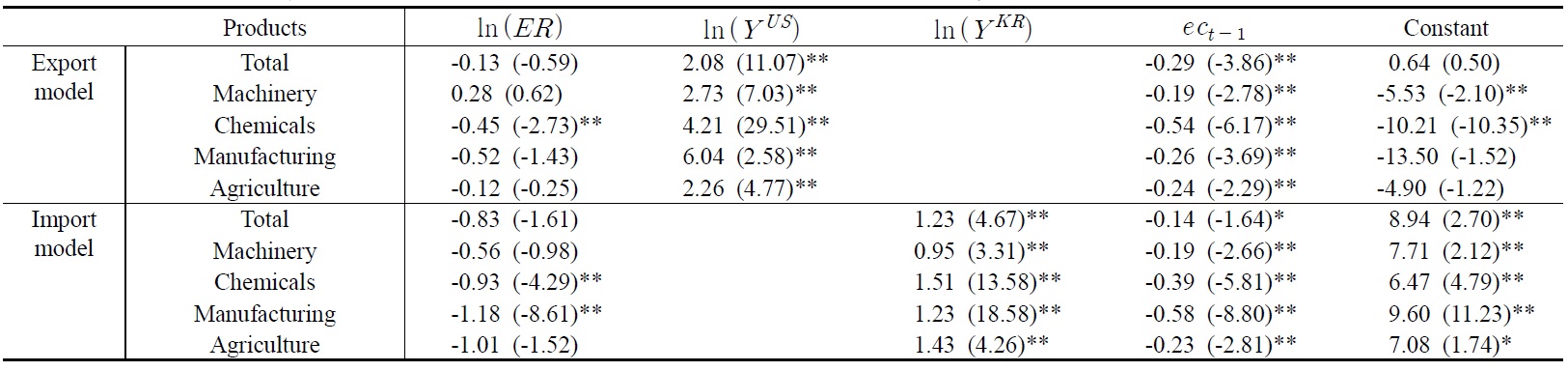
It should be noted that, as discussed earlier, if we employ aggregate data in examining the exchange rate effect on trade flows, our empirical findings may suffer from aggregation bias of data because, among other things, significant coefficients on exchange rate in some industries could be more than offset by insignificant coefficients in others, and vice versa. To shed some light on the argument, therefore, we also estimate equations (5) and (6) using aggregated data of the exports and imports.
5The results of the short-run analysis are not reported here for brevity, but can be obtained from the authors on request. 6We thank the anonymous referees for raising this issue discussed here.
The main purpose of this study is to examine the dynamic interrelationship between changes in exchange rates and changes in Korea’s trade. Although the literature on the relationship between the exchange rate and Korea’s trade exists, relatively little attention has been paid to the direct effects of exchange rates on Korea’s exports and imports at the bilateral commodity/industry level. To fill the gap, we have attempted to assess the effect of exchange rate fluctuations on trade flows in the context of disaggregating the bilateral trade data of 71 industries between Korea and the United States. To achieve this goal, we use the ARDL approach and consider separating the analysis of exports and imports in order to accurately measure the effects of exchange rate changes on bilateral trade. We find that Korean exports are highly sensitive to U.S. income and less by exchange rate changes in both the short- and long-run. On the other hand, it is found that Korean imports are driven largely by the income of Korea and, to some extent, by the bilateral exchange rate. Finally, the empirical results produced by aggregated data of exports and imports are at odds with our findings of disaggregated data, providing partial evidence of the aggregation bias problem. This finding thus explains why it is important to use disaggregating industry data in bilateral export and import models.
[Table 1] Bilateral Commodity Trade between Korea and the United States, 2005-09 Average (million $)

Bilateral Commodity Trade between Korea and the United States, 2005-09 Average (million $)
[Table 2] Results of the F-test for Cointegration among Variables
Results of the F-test for Cointegration among Variables
[Table 3] Estimated Long-run Coefficients of Export Functions of Korea
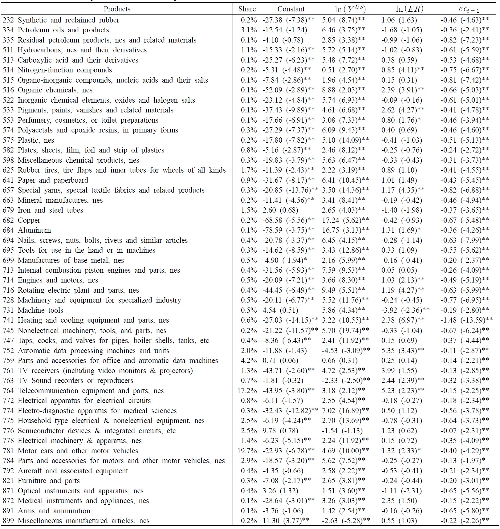
Estimated Long-run Coefficients of Export Functions of Korea
[Table 4] Estimated Long-run Coefficients of Import Functions of Korea
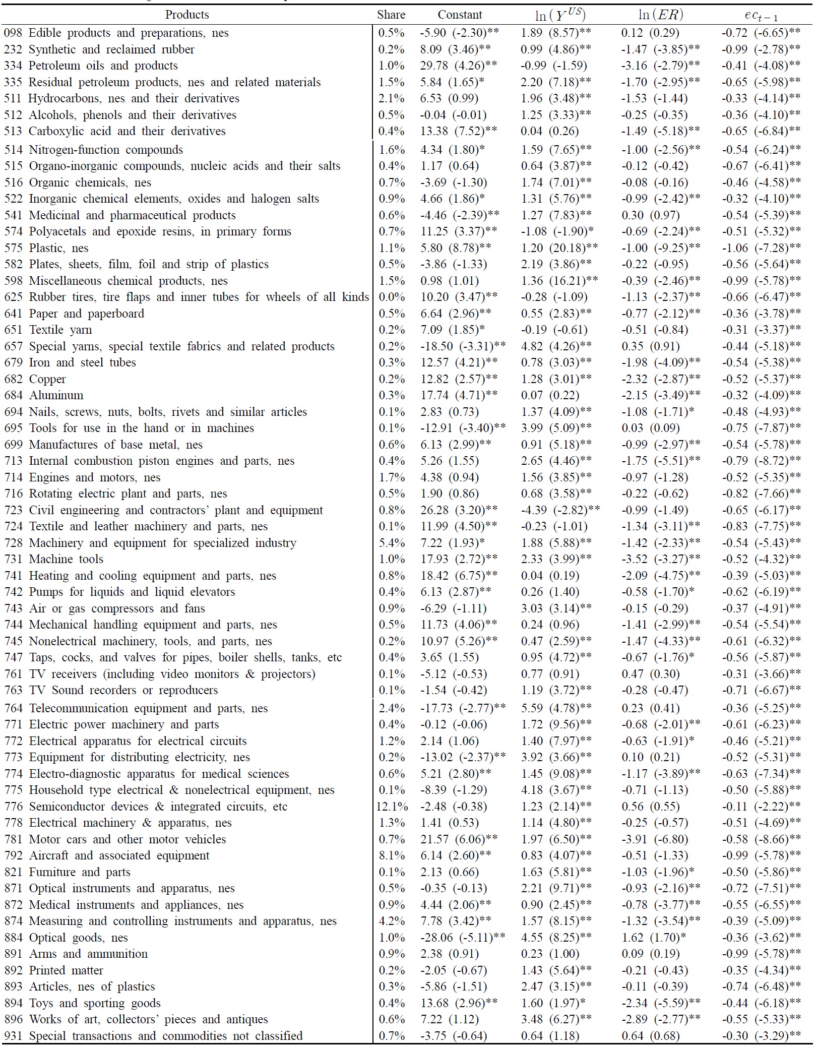
Estimated Long-run Coefficients of Import Functions of Korea
[Table 5] Estimated Long-run Coefficients of Export and Import Functions using Aggregate Data

Estimated Long-run Coefficients of Export and Import Functions using Aggregate Data