검색 전체 메뉴
PDF
맨 위로
OA 학술지
Endogenous Structural Breaks and Real Exchange Rate Stationarity in Asia: Empirics and Theory
  • 비영리 CC BY-NC
ABSTRACT
Endogenous Structural Breaks and Real Exchange Rate Stationarity in Asia: Empirics and Theory
KEYWORD
Real exchange rate , Purchasing power parity , LM unit root test , Structural breaks , New Keynesian model
  • Ⅰ. Introduction

    Purchasing power parity (PPP) as an exchange-rate determination model seems to strike back recently after going through the dark ages of voluminous disastrous empirical testing on its validity1. The central question of the debates concerning PPP reversion now has largely been directed toward the search of trend-stationary real exchange rates2. One interesting strand of literature that inspects the stationarity of real exchange rates is about the use of more satisfactory econometric techniques, out of which the test of the unit root null with structural breaks tops the list3.

    The allowance for structural breaks in testing for PPP is not entirely new. Of late, the empirical testing of the unit-root null with structural breaks in searching for strong evidence of PPP has shed its lights on the East and Southeast Asian currencies, which evidently fulfill the treatment of structural breaks, especially in the aftermath of the currency crash in 1997/98. For instance, Wu et al. (2004) find evidence of stationarity in the real exchange rates among Pacific Basin countries after taking into account a one-time structural change in panel data unit root tests. Zurbruegg and Allsopp (2004), by incorporating structural breaks within a multivariate cointegration structure, show evidence supportive of PPP. Likewise, Fujii (2002) suggests that the effects of the Asian crisis can be generally regarded as a temporary deviation rather than a fundamental shift in real exchange rate behavior. Applying Perron (1989)’s structural unit root test, Aggarwal et al. (2000) find clear and significant evidence in favor of PPP for most of the Southeast Asian currencies in terms of Japanese yen only when the presence of structural breaks in the series is taken into account.

    Although there is mounting evidence of stationary real exchange rates, the evidences remain indecisive due to the potential pitfall of arbitrary predetermining the threshold value and time period of a structural break out of the data-generating-process, as in the tradition of Perron (1998). In previous studies, Zivot and Andrew (1992) caution that a simple inspection of the breakpoint based on data observation can be misleading as sudden changes in data can be mistakenly interpreted as realization from the tail of distribution of the underlying data generating process. One should call this exogeneity into question for  a very basic concern: how likely it is to overlook other breaks not observably as apparent as a nose-diving currency crash, yet significant in reverting the real exchange rates to the parity?

    Subsequently, Zivot and Andrew (1992), Perron (1997), Vogelsang and Perron (1998), to name a few among many others, propose a unit root testing procedure with break points that are not known a priori, but are, instead, determined endogenously. Still, one common issue with such endogenous breaks tests is that they assume no break under the unit root null and derive the critical values accordingly. Lee and Strazicich (2001, 2003) have convincingly argued that the assumption of no breaks under the unit root null in conjunction with an alternate that assumes a unit root with breaks can lead to ‘spurious rejection’. The rejection of the null can be attributed to the presence of a structural break, rather than the stationary alternative. Also, they notice that these tests tend to identify the break point at one period earlier to the true break point, which, in turn, leads to greater ‘spurious rejection’ as the bias in estimating the persistent parameter is maximized.

    Consistent with this line of thought, the objective of this paper is to revisit the test of the unit-root null in the presence of structural breaks in two directions. First, at the empirical front, this paper attempts to expand the literature by allowing for more than one endogenously determined structural break in unit root testing. Ben-David et al. (2003) caution that incorporating one structural break when there are indeed two can as erroneously result in a non-rejection of the unit-root null as in the case of ignoring a break when there is indeed one (see also Lumsdaine and Papell, 1997). Given the relative long span of our sample data, it is likely that the observed unit-root behavior of PPP can be due to the failure of considering for more than one structural break (see Maddala and Kim, 2003). To this end, we use Lee and Strazicich (2001, 2003)’s minimum Lagrangian Multiplier (LM) unit root test that accounts for two structural breaks in null4.

    Second, at the theoretical front, the idea of a structural break captured by means of econometrics without justifying the structural properties seems to be theoretically ill-defined. This paper contributes to the literature by laying out an open-economy New Keynesian model to more systematically characterize the sources of structural breaks and mechanism of a unit root in the real exchange rate. Most interestingly, the model attributes nonstationarity in real exchange rates to the optimally conducted monetary policy for inflation targeters like Korea in conjunction with an endogenous currency risk premium.

    The subsequent discussion is organized as follows. Section 2 reviews the idea of PPP, elaborates on the inappropriateness of existing testing procedures, and illustrates our modeling strategy. We discuss the main results in Section 3. It is then followed by a formalization of structural breaks in Section 4. Section 5 concludes.

    1The classic Rogoff (1996), based on the numerous disappointing results of the empirical validation of PPP, reached a rather gloomy assessment that PPP theory is ‘something of an embarrassment’. A more recent Taylor and Taylor (2004), however, conclude that long-run PPP may hold in the sense that there is significant mean reversion in the real exchange rates, despite the fact that short-run PPP does not hold. To see the flow of development over the years in finding PPP, one can refer to Froot and Rogoff (1995), Sarno and Taylor (2002) , and Taylor (2006).  2See Taylor (2006) for a non-exhaustive list of recent works. It includes Holmes (2010), which allows for Markov switching between a non-stationary and stationary regime, and between stationary regimes with different degrees of persistence. Also included are Baharumshah et al. (2010) who emphasize the nonlinearity in a mean-reverting process of real exchange rates, Ho et al. (2009) who couple real exchange rate stationarity to geographical factors and variability in inflation and nominal exchange rates, and Kocenda (2005) who allows for a single endogenous break in real exchanges.  3Nonlinearity in a mean reversion process of real exchange rates has been another competitive candidate. One can see, for instance, Taylor and Taylor (2004), Taylor (2006), Baharumshah et al. (2010) for the pros of the nonlinearity approach.  4One of the most fascinating advantages of the LM test over other unit-root tests with structural breaks is that it has a test statistic that is invariant to the breakpoint nuisance parameter and thus does not require the assumption of no break(s) under the null to ensure that the test statistic is invariant to breakpoint nuisance parameters, as other tests did.

    Ⅱ. Testing for Real Exchange Rate Stationarity

    The purchasing power parity (PPP) hypothesizes that exchange rates between two currencies adjust to reflect domestic and foreign price levels (in logarithm):

    image

    where

    image

    correspondingly refer to the foreign and domestic price levels, and st denotes the spot nominal exchange rate, defined as home per unit of foreign currency. Early simple regression tests of absolute PPP that corresponds to Eq. (1) is given by

    image

    where ϵt is a disturbance term. A simple test for the absolute PPP is all about testing the null of β1 = 1. On top of that, one can test a less strict form of PPP, known as relative PPP:

    image

    where Δ denotes change in the variable. The null is β0 = 0, β1 = 1. Notwithstanding the simplicity and intuitive appeal of Eq. (3), the critical weakness is the failure to deal with the possibility of nonstationary exchange rates and prices, which, therefore, prompts an alternative approach that evaluates the stationarity of real exchange rates.

    The real exchange rate qt that measures the deviation of st from purchasing power parity can be defined as follows:

    image

    The coefficient β1 = 1 is now imposed and not estimated. PPP holds if qt is identical to zero or a constant. Thus, the idea of PPP is closely related to the stationarity of real exchange rate. While real exchange rates may be subject to considerable short-run variation, the necessary condition for the PPP to hold in the long run is a stationary real exchange rate over time. Putting it formally, the conditional expectation of the long-run real exchange rate tends to be zero.

    image

    where It is the information set available at time t. Accordingly, shocks to real exchange rate disappear as the time horizon expands. Therefore, the autoregressive representation of qt must have no unit root.

    That said, we consider the following data generating process with a p-order autoregressive process to implement a test on the stationarity of the real exchange rate:

    image

    where the error term ϵt follows a white noise process. As shocks are transitory, the real exchange rate will settle down to its long run equilibrium level q* , such that

    image

    If

    image

    the process that drives qt contains the unit root, implying a permanent shock to the real exchange rate. In consequence, the long-run equilibrium does not exist as division by zero is undefined in Eq. (7). To the contrary, if the unit root hypothesis is rejected and

    image

    shock to the real exchange rate vanishes in the long run at the rate of

    image

    per time period. We reparameterize Eq. (6) to produce the following empirical equation

    image

    The most commonly used test is the augmented Dickey-Fuller (ADF) test proposed by Dickey and Fuller (1981) under the unit root null hypothesis of ρ = 0. Rejection of the null suggests little tendency for deviations from PPP.

    One limitation of the conventional ADF unit root test is the inability to recognize PPP when it actually holds outside the structural shift. Montanes and Clemente (1999), Aggarwal et al. (2000), Narayan (2005), and Papell and Prodan (2006), among many others, have convincingly shown that introducing structural break(s) makes the existence of PPP across countries more transparent. Although the more recent ADF-type unit root test is able to accommodate for multiple endogenous trend breaks (Lumsdaine and Papell, 1997), these tests assume no structural break under the unit root null, and derive the critical values accordingly. Nunes et al. (1997) show that this assumption can result in spurious rejections should there be a break under the null (see also Ben-David et al., 2003).

    Lee and Strazicich (2001) further argue that the ADF-type endogenous break test tends to incorrectly select the break point, and more so should the magnitude of the break increase. At this misspecified break point, the persistence is biasedly maximized, resulting in a spurious rejection of the unit root null. Accordingly, Lee and Strazicich (2003) propose a one-break LM unit root test as an alternative to Zivot-Andrews test, and a two-break LM unit root test for Lumsdaine-Papell test. Contrary to the ADF-type test, the size properties of the LM unit root test are fool proof to the presence of breaks under the unit root null. As such, the LM unit root test, which allows for structural breaks under both unit root null and stationary alternative, is able to obviate the invalid estimation of break points and spurious rejection. For this reason, this paper adopts Lee and Strazicich (2003)’s LM unit root test with two breaks.

       1. LM Unit Root with Two Endogenous Structural Breaks

    Consider Lee and Strazicich (2003)’s procedure that corresponds to Perron (1989)’s Model C that allows for two changes in both level Djt and trend DTjt in the series5, for j = 1,2. The two-break LM unit root test statistic for real exchange rate stationarity can be obtained from the following regression:

    where Δ is the difference operator. The vector of exogenous variables, zt, takes the form [1,t,D1t,Dzt,DT1t,DT2t]′. The dummy for level shift Djt = 1 for TTBj + 1, and zero otherwise. The dummy for trend shift DTjt equals tTBj for tTBj + 1, and zero otherwise. The parameter TBj refers to the time location of the break.

    image

    is a detrended series such that

    image

    for t = 2, ... T.

    image

    denotes coefficients in the regression of Δqt on ΔZt, while q1 and Zt, respectively, represents the first observations of qt and Zt. To account for the autocorrelation problem, the regression is augmented with the lagged dependent variables.

    The unit root null hypothesis Փ = 0 is tested by the t-statistics. The unknown break points TBj, j = 1,2, are determined endogenously by searching over the trimming region of (0.1 T, 0.9 T), where T is the sample size. By denoting the break fractions, λj as TBj/T as T→∞, the LM test statistics are defined as:

    image

    The critical values for the two-break minimum LM unit root test statistics are tabulated in Lee and Strazicich (2003).

    5We do not consider Model B as it is commonly believed that most economic time series can be adequately accommodated by Model A and C. Sen (2003) suggests that Model C yields more reliable estimates as compared to Model A, and the former is thus preferred to the latter when a break point is endogenously determined (see, also, Shively, 2000 and Narayan, 2005). For this reason, we consider only Model C.

    Ⅲ. Results and Discussion

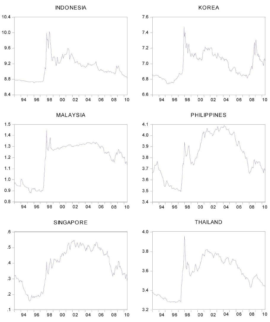
    In this section, we examine the real exchange rates of six East Asian economies, namely Indonesia, Korea, Malaysia, Philippines, Singapore, and Thailand over the time period January 1993 to July 2010. Here, we treat the U.S dollar as the numeraire since the U.S has long been Asia’s major trading partner, particularly as the final destination for regional production, not to speak of its role as the dominant vehicle currency in international trade (Goldberg and Tille, 2008)6. To construct real exchange rates as defined in Eq. (4), monthly data on average market nominal exchange rates and the consumer price index are extracted from the International Financial Statistics (IFS) data bank.

    Figure 1 illustrates the variability of real exchange rates for six Asian economies throughout the years of 1993 and 2010. The sudden and drastic upsurge in real exchange rates during the Asian crisis apparently dominates the scene, suggesting a potential structural shift in the mean and trend of the data after 1997. It is thus interesting to know whether Asian real exchange rates are characterized by unit roots or is indeed trend-stationary that is just subject to structural breaks. Equally fascinating is the fact that, to find another break without hesitation through an informal eyeballing of Figure 1, is barely possible. This difficulty suggests that allowing the breaks to be endogenously determined is a sensible implementation.

    We begin the empirical analysis with the ADF test that serves as a benchmark for comparison. The test includes a deterministic trend to accommodate the potential time trends in the relative consumer prices driven by Balassa- Samuelson effect. Using the ‘general-to-specific’ recursive t-statistics procedure, we set the maximum value of k equal to 12 and use the approximate 10% critical value of 1.645 from the asymptotic normal distribution to assess the significance of the last lag. Ng and Perron (1995) demonstrate that such a ‘t-sig’ approach produces test statistics that perform better in terms of size and power than information-based criteria such as the Akaike information Criterion or the Schwartz Bayesian Criterion. The results from the ADF test, with and without a trend, are reported in Table 1.

    [Table 1] ADF Test Results

    label

    ADF Test Results

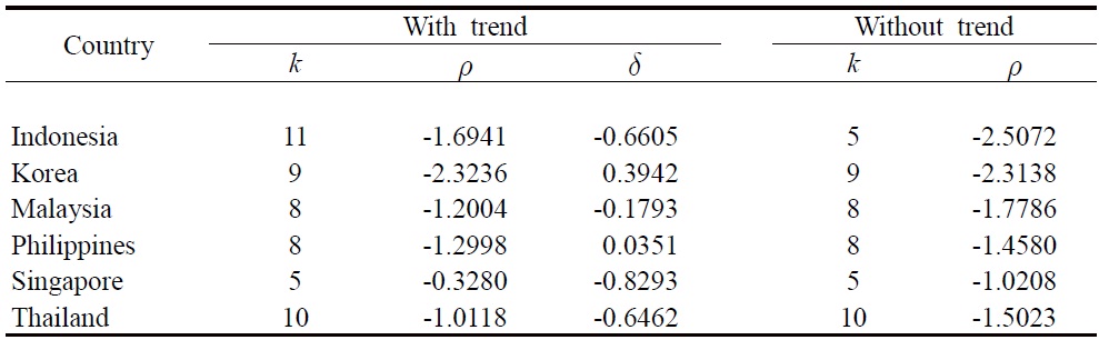
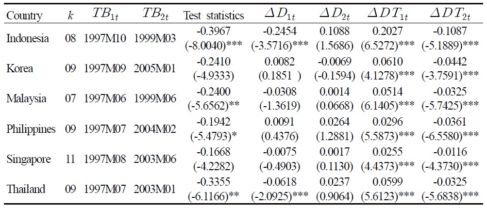
    As expected, the unit root null cannot be rejected. One typical response to such findings is to fault the tests for their lack of power. But as noted previously, the failure to incorporate structural changes in testing the unit root of a time series is too often biased toward finding nonstationarity (see Rappoport and Reichlin, 1989). In view of the potential instability of the PPP relationship associated with exceptional events like the onset of Asian currency crisis, unit root tests that permit level and trend breaks are naturally sensible for analyzing the long run behavior of the real exchange rates. Indeed, by applying the LM unit root test with two endogenous breaks, we find evidence in favor of the PPP hypothesis. The results of the two-break LM unit root test are presented in Table 2.

    [Table 2] Two-break LM Tests

    label

    Two-break LM Tests

    Table 2 reveals that the unit root null can be rejected in favor of the trend-break stationary alternative for four of the six real exchange rates (Korea and Singapore are the exceptions), out of which three are at least at a 5% significant level. As the minimum LM tests assume breaks under the null, rejection of the unit root null profoundly confirms that the real exchange rates of  these Asian countries are trend-stationary and are subject to structural change. Interestingly, the results also indicate that a trend break is statistically more critical than a level-break in accounting for real exchange rate stationarity.

    Because the minimum LM test endogenizes the determination of break points, the outcome is foolproof to the criticism of arbitrarily imposed break dates (Christiano, 1992). The first estimated break points collectively appear within June and October of 1997. This finding is certainly consistent with the onset of the Asian currency and financial crises since July 1997. More puzzling is the heterogeneous second estimated break points that fall unsystematically in between 2003 and 2005. Unlike the first estimated break points, these second estimated breaks are not cursorily observable in the figure, which of course substantiates the importance of endogeneity in break determination. Of further interest is whether a mechanism that is able to consistently account for this variety of break points can be found.

    6Baharumshah et al. (2007) showed that mean reversion of real exchange rates in the framework of a panel unit root test without break for a set of countries exactly identical to ours appears to be invariant to the choice of the numeraire currency. Nusair (2008) also concludes that base currency is not critical to the finding of long-run PPP.

    Ⅳ. An Interpretation of Structural Breaks in the New Keynesian Model

    Conceptually, the path of real exchange rates (in logarithm) can be described as

    image

    where q* denotes the steady-state real exchange rate, and ϵt~iid(0,σ2) is stochastic white noise. Let

    image

    We can augment Eq. (11) to conceptually resemble Perron (1989)’s Model C of structural break (ignoring time trend and constant):

    image

    where Dp and DL, respectively, denote a pulse dummy (mean break) and level dummy (level break). In line with Eq. (8) in section II, Eq. (12) indicates that a temporary innovation can end with a permanent deviation of the real exchange rate from its steady state if ρ ≥ 1. It is thus of interest to figure out the structural meaning of ρ. Besides, what constitutes a pulse dummy and level dummy? Can we structurally define μ1 and μ2? To this end, we set up a simple open-economy New Keynesian model to provide a body of analytics for inspecting the mechanism of breaks in real exchange rates.

       1. A New Keynesian set-up

    Consider an economy with working households endowed with one-period state-contingent bonds. Human and non-human incomes finance non-storable consumption and purchase of assets. Household’s problem, therefore, can be written as to maximize the discounted future streams of utility,

    image

    subject to the budget constraint

    image

    where β is the discounted rate.

    image

    is the real exchange rate, Փ(St–1 is risk premium that is increasing with the level of nominal exchange rate. Փ′(St–1>0 indicates that the current level of nominal exchange rate will influence the prospective risk premium of the currency, which in turn affects the path of future nominal exchange rates.

    On top of that, bt and

    image

    respectively, denote real domestic and foreign bonds that pay real yields. Wt is real wage and Nt is hours worked. The parameter σ is the coefficient of relative risk aversion. The reciprocal thus denotes the elasticity of substitution between consumptions at t and t + 1. For the sake of simplicity without implication, we assume a unitary wage elasticity of the labor supply. Consumption goods are a composite of home and imported foreign goods

    image

    where

    image

    and

    image

    Derived from the first-order conditions, the marginal rate of substitution between consumption and hours worked is given by

    image

    Besides, the consumer’s optimality condition with respect to intertemporal consumption allocation can be derived as

    image

    where it is nominal interest rate, and Pt is price level. Under the assumption of a complete securities market, Eq. (17) holds equally for the foreign representative consumer. Taken together with arbitrage in securities that assures international risk sharing

    image

    and the definition of real exchange rate, we can get

    image

    Consider now a simple production function of firm j with time-to-hire labor.

    image

    By denoting the shadow price of the Lagrangian problem as real marginal cost (RMCt), a firm’s cost minimization problem gives the following optimal condition.

    image

    Firm j has to choose

    image

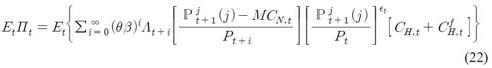
    in order to maximize the expected discounted profits (Ett) in the form

    image

    where θ is the probability that firm j is not able to adjust its price. t+i satisfies

    image

    denotes the discounted factor in the interest of households. MCn,t is the consumer-good producer’s nominal marginal cost, and

    image

    is home export. Eq. (22) assumes producer currency pricing in exporting, and the pricing decision is symmetrical for all firm j in equilibrium.

    In a Calvo price setting, firms that receive signals at probability 1 – θ for price reoptimization will reset prices to the approximate optimal reset price

    image

    derived from Eq. (22). Those that have not received the signal at probability θ will follow with the last-period price, out of which a fraction will index their new price to the last-period inflation. Since the aggregate log price level at each date is a probability-weighted average of partially indexed aggregate log price levels and newly reset prices, the New Keynesian Phillips curve for inflation can be derived as

    image

    To close the model, we assume the following monetary policy function:

    image

    The sum of the first two items on the right hand side amounts to the targeted nominal interest rate. The coefficients vπ,vy,vq and vΔq, respectively, indicate a policy reaction towards the stabilization of inflation, output, and level and changes in real exchange rates. Note that all corresponding behavioral equations derived, ranging from consumption Euler condition to inflation dynamics and monetary policy, are equally applicable for the foreign country.

       2. Deriving the sources of unit root and structural breaks

    Consider the definition of real exchange rate. The log deviation of real exchange rates can be written as

    image

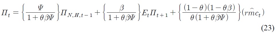
    The inflation differentials in Eq. (25) can be substituted by the difference between the New Keynesian Philips curve of foreign and home economy, which simplifies to

    image

    where

    image

    Next, Pareto efficient allocation ensures that

    image

    Together with the foreign counterpart of Eq. (27) and Eq. (19), Eq. (26) can be further simplified to

    image

    The last resolution is to put monetary policy into Eq. (28). Rearrange the home monetary policy function of Eq. (24) and identical foreign monetary policy function in such a way that

    image

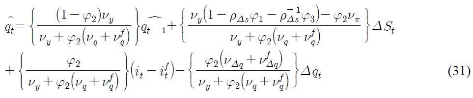
    Substitute Eq. (29) into Eq. (28), we get

    image

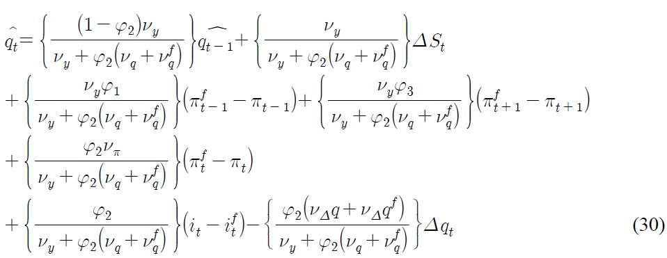
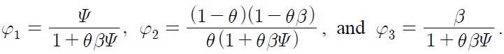
    where further simplification gives us

    image

    Eq. (31) resembles Eq. (12) in that
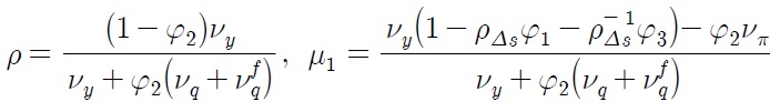
    image

    and

    image

       3. What causes breaks?

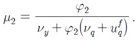
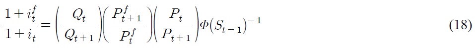
    According to Eq. (30), interest rate differentials

    image

    due to asymmetry in the conduct of monetary policy, constitute the break in the level of real exchange rate, whereas nominal depreciation rate and inflation differentials contribute to the break in steepness of the trend of real exchange rate. The magnitude of each source of break depends on the degree of price stickiness, which influences the value of φi, and policy reaction toward targeted variables. Although it is beyond our scope to provide precise quantitative estimates of the strength of each source, some simple simulations on Eq. (30) allow us to infer to what extent nominal rigidities and the conduct of monetary policy would have affected the potential occurrence of breaks.

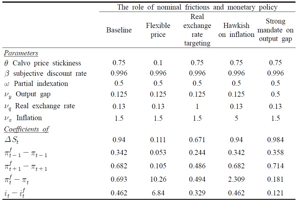
    In particular, results contained in Table 3 show that:

    [Table 3] Effects of Nominal Rigidities and Monetary Policy in Generating Structural Breaks

    label

    Effects of Nominal Rigidities and Monetary Policy in Generating Structural Breaks

       4. Explaining nonstationary real exchange rate

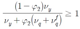
    Can our model explain why the unit root null hypothesis for the case of Korea, for instance, cannot be rejected even when breaks are accounted for? The answer lies in Eq. (30). As real exchange rate is described as a unit-root process if ρ ≥ 1, we get

    image

    which simplifies to

    image

    Sanchez (2009) has interestingly found that the Bank of Korea places negligible emphasis on both output and the exchange rates. This implies vq, vy ≈ 0. Based on Eq. (32), it can be easily seen then that the condition characterizing unit-root process in the real exchange rate is met once the foreign counterparts of the Bank of Korea smooth exchange rate fluctuations,

    image

    And what matters the most is vq not vy.

    The intuition is straightforward, particularly for inflation targeters like Korea. Let us rewrite Eq. (24) in terms of output gap

    image

    where

    image

    denotes the log deviation of natural output from its steady state. Suppose there is a productivity progress that increases the natural output over the steady state, and the variance of the productivity shock ϵt is increasing in the absolute value of vy. Positive deviation of the natural output on the one hand calls for a rise in interest rate, the resultant widening output gap on the other hands needs a fall in interest rate. These forces counterbalance each other, leaving no room for an output gap in the conduct of monetary policy, irrespective of the value of vy. So vy doesn’t matter in real exchange rate nonstationarity.

    On the other hand, as price tends to fall in the aftermath of a favorable productivity shock, the optimal monetary response for inflation targeters like Korea requires a contemporaneous fall in interest rate to accommodate the rise in natural output. Put in our context, a fall in nominal and thus real interest rate below a long-run average, given the sticky-price environment, causes a level-break in real exchange rates. Because real depreciation is expansionary and facilitates a central bank’s task to close the output gap in order to stabilize the inflation, inflation targeters can be tolerant of real depreciation such that vq=0. According to Eq. (18), nominal depreciation will increase the prospective risk premium of the currency, resulting in a level of nominal and real exchange rates that can be persistently above the long-run average. The more successful the central bank is in stabilizing the inflation fluctuation, the more persistent the real exchange rates will be. In short, the conduct of an optimal monetary policy for inflation targeters that ignores real exchange rate stabilization can potentially be the culprit of unit root behavior in real exchange rates, despite the consideration of endogenous breaks.

    Ⅴ. Conclusion

    This paper reconsiders real exchange rate stationarity in the framework of the minimum Lagrangian Multiplier unit root test that can account for two endogenously determined structural breaks. Allowing for endogenous break determination and explicit consideration of breaks under the unit root null have been the two main pillars that make this procedure the most appropriate one in testing for real exchange rate stationarity. Our results are mixed. Some exhibit trend-stationary real exchange rates, while some others did not. This motivates us to address two important questions: What constitutes structural breaks? And  what drives the unit root process?

    By shedding lights on a simple New Keynesian model, we conjecture that an interest rate differential is the source of a level-break, whereas the rate of nominal depreciation and inflation differentials can instigate a mean-break. The magnitude of each factor is largely influenced by the degree of price stickiness and the central bank’s preference toward inflation, output and real exchange rate stabilization. We further show that the conduct of monetary policy that places negligible emphasis on real exchange rate moderation can result in nonstationary real exchange rates, particularly when the currency risk premium is increasing in the level of nominal exchange rates.

    What is particularly important, but is out of the scope of this paper and thus is of interest for future study, is certainly the quantitative evaluation of the model of real exchange rate nonstationarity based on individual country experience. Because persistent deviation of real exchange rates from the long-run average can end with crisis-provoking resource misallocation, probing into the relationship between optimal monetary policy and real exchange rate nonstationarity shall be a promising venue for future study.

참고문헌
  • 1. Aggarwal R., Montanes A., Ponz M. (2000) “Evidence of Long-Run Purchasing Power Parity: Analysis of Real Asian Exchange Rates in terms of the Japanese Yen” [Japan and the World Economy] Vol.12 P.351-361 google cross ref
  • 2. Baharumshah A. Z., Aggarwal R., Chan T. -H. (2007) “East Asian Real Exchange Rates and PPP: New Evidence from Panel Data Tests” [Global Economic Review] Vol.36 P.103-119 google cross ref
  • 3. Baharumshah A. Z., Liew V.K. -S., Chowdhury I. (2010) “Asymmetry Dynamics in real exchange rates: new results on East Asian currencies” [International Review of Economics and Finance] Vol.19 P.648-661 google cross ref
  • 4. Ben-David D., Lumsdaine R., Papell D. H. (2003) “Unit Root, Postwar Slowdowns and Long-Run Growth: Evidence from Two Structural Breaks” [Empirical Economics] Vol.28 P.303-319 google cross ref
  • 5. Christiano L. (1992) “Searching for A Break in GNP” [Journal of Business and Economic Statistics] Vol.10 P.237-250 google
  • 6. Dickey D. A., Fuller W. A. (1981) “Likelihood Ratio Statistics for Autoregressive Time Series with A Unit Root” [Econometrica] Vol.49 P.1057-1072 google cross ref
  • 7. Froot K. A., Rogoff K. (1995) “Perspectives on PPP and long-run real exchange rates,” in: Rogoff, K. and G. Grossman (Eds.), Handbook of International Economics google
  • 8. Fujii E. (2001), “Exchange Rate and Price Adjustments in the Aftermath of the Asian Crisis” [International Journal of Finance and Economics] Vol.7 P.1-14 google cross ref
  • 9. Goldberg L., Tille C. (2008) “Vehicle Currency Use in International Trade” [Journal of International Economics] Vol.76 P.177-192 google cross ref
  • 10. Ho C.-C., Cheng S.-Y., Hou H. (2009) “Purchasing Power Parity and Country Characteristics: Evidence from Time Series Analysis” [Economics Bulletin] Vol.29 P.444-456 google
  • 11. Holmes M. J. (2010) “Are Asia-Pacific Real Exchange Rates Stationary? A Regime-Switching Perspective” [Pacific Economic Review] Vol.15 P.189-203 google cross ref
  • 12. Kocenda E. (2005) “Beware of Breaks in Exchange Rates: Evidence from European Transition Countries” [Economic System] Vol.29 P.307-324 google cross ref
  • 13. Lee J., Strazicich M. (2001) “Break Point Estimation and Spurious Rejections with Endogenous Unit Root Tests” [Oxford Bulletin of Economics and Statistics] Vol.63 P.535-558 google cross ref
  • 14. Lee J., Strazicich M. (2003) “Minimum LM Unit Root Test with Two Structural Breaks” [Review of Economics and Statistics] Vol.85 P.1082-1089 google cross ref
  • 15. Lumsdaine R., Papell D. (1997) “Multiple Trend Breaks and the Unit Root Hypothesis” [Review of Economics and Statistics] Vol.79 P.212-218 google cross ref
  • 16. Maddala G. S., Kim I. M. (2003) Unit Root, Cointegration and Structural Change. google
  • 17. Montanes A., Clemente J. (1999) “Real Exchange Rates and Structural Breaks: Evidence for Spanish Peseta [Applied Economics Letters] Vol.6 P.349-352 google cross ref
  • 18. Narayan P. K. (2005) “New Evidence on Purchasing Power Parity from 17 OECD Countries” [Applied Economics] Vol.37 P.1063-1071 google cross ref
  • 19. Ng S., Perron P. (1995) “Unit Root Tests in ARMA Models with Data-Dependent Methods for the Selection of the Truncation Lag” [Journal of the American Statistical Association] Vol.90 P.269-281 google cross ref
  • 20. Nunes L., Newbold P., Kuan C. (1997) “Testing for Unit Roots with Breaks: Evidence on the Great Crash and the Unit Root Hypothesis Reconsidered” [Oxford Bulletin of Economics and Statistics] Vol.59 P.435-448 google cross ref
  • 21. Nusair S. A. (2008) “Purchasing Power Parity under Regime Shifts: An Application to Asian Countries” [Asian Economic Journal] Vol.22 P.241-266 google cross ref
  • 22. Papell D. H., Prodan R. (2006) “Additional Evidence of Long-Run Purchasing Power Parity with Restricted Structural Change” [Journal of Money, Credit, and Banking] Vol.38 P.1329-1349 google cross ref
  • 23. Perron P. (1989) “The Great Crash, the Oil Shock and the Unit-Root Hypothesis” [Econometrica] Vol.57 P.1361-1401 google cross ref
  • 24. Perron P. (1997) “Further Evidence on Breaking Trend Functions in Macroeconomic Variables” [Journal of Econometrics] Vol.80 P.355-385 google cross ref
  • 25. Rogoff K. (1996) “The Purchasing Power Parity Puzzle” [Journal of Economic Literature] Vol.34 P.647-68 google
  • 26. Rappoport P., Reichlin L. (1989) “Segmented Trends and Non-Stationary Time Series” [Economic Journal] Vol.99 P.168-177 google cross ref
  • 27. Sanchez M. (2009) “Characterising Inflation Targeting Regime in South Korea” google
  • 28. Sarno L., Taylor M. (2002) “Purchasing Power Parity and the Real Exchange Rate” [IMF Staff Paper] Vol.49 P.65-104 google
  • 29. Sen A. (2003) “On Unit Root Tests When the Alternative Is a Trend Break Stationary Process” [Journal of Business and Economic Statistics] Vol.21 P.174-184 google cross ref
  • 30. Shively P. A. (2000) “A Test of Long Run Purchasing Power Parity” [Economics Letters] Vol.73 P.201-205 google cross ref
  • 31. Taylor A. M., Taylor M. P. (2004) “The Purchasing Power Parity Debate” [Journal of Economic Perspective] Vol.18 P.135-158 google cross ref
  • 32. Taylor M. P. (2006) “Real Exchange Rates and Purchasing Power Parity: Mean Reversion in Economic Thought” [Applied Financial Economics] Vol.16 P.1-17 google cross ref
  • 33. Vogelsang T. J., Perron P. (1998) “Additional Tests for a Unit Root Allowing for a Break in the Trend at an Unknown Time” [International Economic Review] Vol.39 P.1073-1100 google cross ref
  • 34. Wu J. L., Tsai L. J., Chen S. L. (2004) “Are Real Exchange Rates Non-Stationary? The Pacific Basin Perspective” [Journal of Asian Economics] Vol.15 P.425-438 google cross ref
  • 35. Zivot E., Andrews D.W.K. (1992) “Further Evidence on the Great Crash, the Oil-Price Shock, and the Unit-Root Hypothesis” [Journal of Business and Economics Statistics] Vol.10 P.251-270 google
  • 36. Zurbruegg R., Allsopp L. (2004) “Purchasing Power Paity and the Impact of the East Asian Currency Crises” [Journal of Asian Economics] Vol.15 P.739-758 google cross ref
이미지 / 테이블
  • [ ] 
  • [ ] 
  • [ ] 
  • [ ] 
  • [ ] 
  • [ ] 
  • [ ] 
  • [ ] 
  • [ ] 
  • [ ] 
  • [ ] 
  • [ ] 
  • [ ] 
  • [ ] 
  • [ ] 
  • [ ] 
  • [ Figure 1 ]  Real Exchange Rates (in natural logarithms), 1993:M01 ? 2010:M07
    Real Exchange Rates (in natural logarithms), 1993:M01 ? 2010:M07
  • [ Table 1 ]  ADF Test Results
    ADF Test Results
  • [ Table 2 ]  Two-break LM Tests
    Two-break LM Tests
  • [ ] 
  • [ ] 
  • [ ] 
  • [ ] 
  • [ ] 
  • [ ] 
  • [ ] 
  • [ ] 
  • [ ] 
  • [ ] 
  • [ ] 
  • [ ] 
  • [ ] 
  • [ ] 
  • [ ] 
  • [ ] 
  • [ ] 
  • [ ] 
  • [ ] 
  • [ ] 
  • [ ] 
  • [ ] 
  • [ ] 
  • [ ] 
  • [ ] 
  • [ ] 
  • [ ] 
  • [ ] 
  • [ ] 
  • [ ] 
  • [ ] 
  • [ ] 
  • [ ] 
  • [ ] 
  • [ Table 3 ]  Effects of Nominal Rigidities and Monetary Policy in Generating Structural Breaks
    Effects of Nominal Rigidities and Monetary Policy in Generating Structural Breaks
  • [ ] 
  • [ ] 
  • [ ] 
  • [ ] 
  • [ ] 
(우)06579 서울시 서초구 반포대로 201(반포동)
Tel. 02-537-6389 | Fax. 02-590-0571 | 문의 : oak2014@korea.kr
Copyright(c) National Library of Korea. All rights reserved.