Ⅰ. Introduction and Background
Highly fluctuating exchange rate since the collapse of the Bretton Woods system of fixed exchange rates in the early 1970s has led to a number of studies examining the effects of exchange rate volatility on export flows. Exports respond to a number of variables such as foreign income as well as the exchange rate and its volatility. Although there is a broad consensus on the effects of foreign income and the exchange rate on exports, previous theoretical and empirical studies have provided inconsistent findings on the impact of exchange rate volatility on international trade. At the theoretical level, some studies have presented models showing how exchange rate volatility may exert positive or negative effects on trade (e.g., Artus, 1983; Brodsky, 1984; De Grauwe, 1988; Franke, 1991; Dallas and Zilberfarb, 1993; Secru and Raman, 2000; Baccheta and van Wincoop, 2000). At the same time, empirical studies have also provided mixed results with respect to the evidence that world trade data typically fails to reveal a consistent relationship between exchange rate volatility and trade (e.g., Chowdhury, 1993; Bahmani-Oskooee and Payesteh, 1993; Aristotelous, 2001; Tenreyro, 2004; De Vita and Abbott, 2004). Previous studies examining the relationship between exchange rate volatility and trade flows, such as Mckenzie (1999) and Bahmani-Oskooee and Hegerty (2007), suggest that fundamental ambiguities remain.
As the mass of international trade flows between developed countries, most of the previous theoretical and empirical studies examining the effects of exchange rate volatility have focused on the experiences of developed economies in Western Europe and North America (De Grauwe and Bellefroid, 1986; Mckenzie, 1999). However, as Mckenzie (1999) mentioned, few studies have focused on less developed countries. For instance, Onafowora and Owoye (2008) recently examined the impact of exchange rate volatility on Nigeria’s exports to the U.S. by using the cointegration and vector error correction model (VECM) framework. This paper presents further evidence of the impact of exchange rate volatility on trade flows by focusing on Korea, a recently developed and export-oriented economy, and provides valuable insights into the relationship between exchange rate volatility and exports in small open economies.
This study is different from previous studies in the way of considering the hypothesis of the
The asymmetry through the first channel may also occur due to asymmetric pricing-to-market (PTM) behavior, which involves adjusting export prices based on the degree of competition in foreign markets. Marston (1990) and Knetter (1994) have focused on asymmetric PTM, which is greater with appreciations than depreciations. They argue that exporting firms with market share objectives do not permit foreign currency prices to increase when the domestic currency appreciates. Rather than pass on the effects of the appreciation by raising foreign currency prices and risk losing sales volume, exporting firms maintain foreign currency prices and effectively reduce domestic profit margins. In contrast, PTM occurs to a lesser extent with domestic currency depreciations. Thus, the asymmetric PTM hypothesis reflects the foreign exchange market’s asymmetric behavior and the asymmetric effect with respect to exchange rate uncertainty during appreciations and depreciations.
The asymmetry through the second channel means that the exchange rate fluctuates differently while it appreciates and depreciates, resulting in the asymmetric volatility of the exchange rate movement, which reflects the foreign exchange market’s asymmetric behavior with respect to exchange rate risk. For the exchange rate, it is often observed that the market responds to exchange rate volatility differently as the exchange rate appreciates or depreciates. This asymmetry in the exchange rate was discovered by Black (1976) and confirmed by subsequent findings. The majority of empirical studies on nonlinear exchange risk exposure have focused on the asymmetric nature of exchange risk exposure over the appreciation-depreciation cycles, and observed that there exist asymmetric effects of exchange rate risk with a dynamic conditional variance (Nelson, 1991; Engle and Ng, 1993; Tse and Tsui, 2002; Koutmos and Martin, 2003) . In other words, the asymmetry through the second channel means that exchange rates are negatively correlated with changes in exchange rate volatility, such that this volatility tends to increase in response to bad news and decrease in response to good news.
This paper considers two effects of this
In addition, this study differs from previous studies in terms of econometric methodology. The recent studies mentioned earlier have typically used timeseries data and approaches such as the cointegration and ECM frameworks. However, such studies have been limited by spurious regression problems because they have not taken into account the integrating properties of individual variables in their models. When testing causality in the export demand function, it is necessary to examine the time-series properties of the individual series concerned because the data used in the estimation are time series data, which means that the series could change over time and do not have fixed or stationary means. The statistical inference from time series analysis is typically based on the integration property of the series. Thus, results obtained without examining the integration of time-series data can be considered as spurious. Previous studies have typically assumed that, like other variables in the model, the measure of exchange rate volatility is integrated of order one, allowing them to apply the cointegration technique (Bahmani-Oskooee and Kovyryalova, 2008). To address this deficiency, the present study focuses on the integration property of individual variables, including the measure of volatility, and applies recent econometric techniques of cointegration, namely the
In sum, to capture and test for asymmetry in the effects of the exchange rate risk on exports and to simultaneously consider the asymmetric conditional variance in volatility, this study uses and applies the bounds testing approach to asymmetric GARCH models. The dynamic dummy variables in the unrestricted error correction model (UECM) capture the asymmetric effect of exchange rate risk on exports, and the asymmetric GARCH specification captures the asymmetry in the conditional variance of exchange rate volatility. Thus, this study estimates the benchmark model and three types of asymmetric GARCH models by applying the bounds testing approach and compares the results to investigate the dynamic impact of the asymmetric effects of exchange rate volatility on Korea’s exports to its major trading partners, the U.S. and Japan, by using quarterly data spanning from 1980 to 2009.
The rest of the paper is organized as follows. Section II discusses the background and methodology of the empirical specification for estimating the export equation and volatility measures. The specification combines the unrestricted error correction framework of the bounds testing approach with asymmetric GARCH models. Section III presents and discusses the data and the empirical results, and Section IV concludes.
There are two primary determinants of export demand (Dornbusch, 1988). One is the foreign income variable, which captures the economic activity and purchasing power of the trading partner country, and the other is the relative price variable for the terms of trade. Thus, previous studies have used standard export demand functions with an economy scale variable and a relative price term. Previous studies have typically added a measure of exchange rate volatility to this function to determine the impact of exchange rate uncertainty on trade flows. The nonstructural reduced-form export equation in previous studies such as Rose (1990), Pozo (1992), Klassen (2004), Onafowora and Owoye (2008), and Bahmani-Oskppee and Kovyryalova (2008), among others, has been a building block for empirically analyzing the effect of exchange rate volatility. Trade theory suggests that an increase in foreign income leads to an increase in the demand for exports. On the other hand, if relative export prices rise, the demand for exports will fall because domestic goods become less competitive than foreign ones. The effect of exchange rate volatility on exports is ambiguous because it depends on traders’ attitudes toward uncertainty (Onafowora and Owoye, 2008). Most of the previous empirical studies have treated exchange-rate uncertainty as a risk. Under the assumption of risk aversion, an increase in the level of risk leads to higher costs for risk-averse traders and also to less trade because exporters would view it as an increase in the uncertainty of profits on international transactions (Aristotelous, 2001). However, risk-neutral or less risk-averse traders are less concerned with extreme outcomes. Moreover, traders may anticipate future exchange-rate movements and gains from this knowledge may offset the risk of exchange-rate uncertainty. Hence, the influence of exchange rate volatility on exports is ambiguous from a theoretical point of view, and is more an empirical matter because it cannot be determined a priori. Thus, the present study uses a benchmark estimation function based on the following long-run real export demand functions from the model specifications used in previous research:

where Xi is the logarithm of real exports, Yi is the logarithm of real foreign income, Pi is the logarithm of the relative export price, Vi is the logarithm of the measure of exchange rate volatility, and
Most of the previous studies involving time-series data have assumed that the measure of exchange rate uncertainty is integrated of order one, like other variables in the model. This allowed such studies to apply cointegration techniques. If all the concerned variables were nonstationary and integrated of the same order, it would be of interest to investigate the useful cointegrating relationships that could form the basis of estimating an error correction model (ECM). Such cointegrating relationships may specify the dynamics in a manner that forces short-run relationships to be consistent with their long-run counterparts. For there to be a cointegrating relationship between these variables, each series must be a unit root and integrated of the same order (Engle and Granger, 1987). In fact, however, Doyle (2001) and others proposed that whereas other variables are non-stationary, real exchange rate volatility and nominal exchange rate volatility are stationary in levels, implying that they play no role in the long-run error correction model. Furthermore, Anderson et al. (2001) and Klaasen (2004) suggested that the conditional variance in exchange rate as a measure of exchange rate volatility is stationary.
These findings imply that either the benchmark relationship or the cointegrating relation in Equation (1) that is proposed in most of the previous studies may reflect the spurious problem because such studies have not taken into account the fact that the volatility variables are typically integrated of different orders from those of other variables in the export equation.
Therefore, to produce empirical results that are more robust and not spurious, this study employs and applies a recent technique called the bounds testing approach, which was introduced by Pesaran et al. (2001), to test the asymmetry hypothesis for short and long-run relations. This technique has an interesting property in which the variables included in the cointegrating space can be either stationary (e.g., a measure of volatility) or non-stationary and there is no need for the same order of integration. In other words, Pesaran et al.’s (2001) technique is more suitable for the present study because, whereas other variables such as exports and income can be non-stationary, the volatility measure for the bilateral exchange rate can be stationary,
The initial step of the bounds testing approach involves using Equation (1) to estimate long-run coefficients with short-run dynamics. This can be expressed as the following error-correction representation, which was developed by Engle and Granger (1987):

where
Next, Pesaran et al. (2001) introduced a relatively new technique in which variables may be I(1) or I(0) in the error-correction model (2). In the equation, they replace the error-correction term

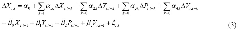
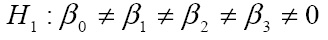
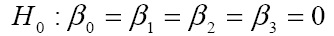
The presence of a long-run relationship among the variables in Equation (3) is determined by using the bounds testing procedure in Pesaran et al. (2001), which is based on the F-statistic for cointegration analysis. They proposed that the asymptotic distribution of the F-statistic is non-standard under the null hypothesis of no cointegration between examined variables regardless of whether explanatory variables are purely I(0) or I(1). They tabulated upper-bound critical values for when all the variables are assumed to be I(1) and lower-bound critical values for when they are I(0). If the calculated F-statistic is greater than the upper bound, then the lagged level variables are jointly significant and must be retained. Thus, a significant F-statistic implies that all variables are cointegrated. To implement the bounds test, the null hypothesis (H0) is tested against an alternative (H1) by considering the unrestricted error correction model for the export demand equation (3) and a joint significance test is performed as follows:

Again, the estimates of
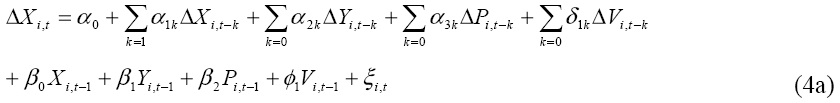
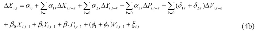
Finally, this study applies Pesaran et al.’s unrestricted error correction model (UECM) framework by introducing dynamic dummy variables into Equation (3) of the bounds testing approach to investigate the asymmetric effect in short and long-run dynamics simultaneously. Then, the bounds testing specification with the dynamic dummies takes the following form:
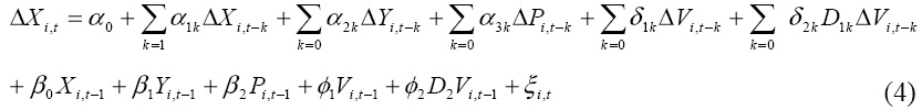
where D1k=1 for appreciation and 0 for depreciation at time t-k, and D2=1 for appreciation and 0 for depreciation of the exchange rate at time t-1. ∑Dlk captures the difference in the effects of exchange rate uncertainty between appreciations and depreciations in short run and D2 captures the difference in the effects in the long run equilibrium
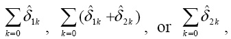
To examine the asymmetric effect of exchange rate volatility on exports, this study tests the hypothesis that the effect of the exchange rate uncertainty differs depending on whether the exchange rate is appreciating or depreciating. Let
Then the estimated relations can be expressed as follows:


where time lags in dummy variables capture the dynamic feature of the asymmetric effect of exchange rate risk on exports, and

measures the short-run difference in the effects of exchange rate risk between appreciations and depreciations of the exchange rate. If either
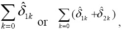
(or both) significantly differ from zero in Equation (4) and if

also differs significantly from zero, then there is statistical evidence for the short-run asymmetric effect. If both sums are insignificant, then exchange rate risk has no effect on exports. It takes a similar procedure to test the hypothesis for the long-run asymmetric effect. Here

or

(or both) in Equation (4) differ significantly from zero and if

also differs significantly from zero, then there is statistical evidence for the long-run asymmetric effect.
Previous empirical research on the influence of exchange rate volatility on exports has raised a number of central issues. The most important issues concern the appropriate measure by which exchange rate volatility may be measured (McKenzie, 1999). Exchange rate volatility is not directly observable, but various statistical measures have been used in previous studies. McKenzie (1999) and Bahmani-Oskooee and Hegerty (2007), among others, presented comprehensive reviews of various measures of exchange rate volatility. Although previous studies have tended to use one measure of exchange-rate volatility by assuming that the error term has a constant variance in estimating the exchange rate process, the present study uses the most recent measures by considering time-varying and asymmetric responses to the volatility of exchange rates.
In this study, exchange rate risk is specified as time-varying volatility and is measured by recently developed methods using the conditional variance in the exchange rate modeled as a GARCH-type process (Engle, 1982; Bollerslev, 1986) and its extensions with asymmetric GARCH models. Hodrick and Srivastava (1984) identified exchange rate risk as conditional and time varying. Unlike traditional measures of exchange rate volatility which may potentially ignore information on the stochastic processes by which exchange rates are generated (Jansen, 1989), GARCH-type models capture the timevarying conditional variance as a parameter generated from a time-series model of the conditional mean and variance, which can be very useful in describing volatility clustering (Onafowora and Owoye, 2008). GARCH models can successfully model the relationship between the variances and means (Bollerslev, 1986; Engle et al., 1987; Bollerslev et al., 1992). Following Bollerslev (1986), the present study specifies exchange rate risk as time-varying exchange rate volatility constructed through the GARCH process so that a larger estimated conditional variance can indicate a higher level of risk. Further, in terms of exchange rates, previous studies have observed that there exist asymmetric effects of exchange rate risk with dynamic conditional variances (e.g., Engle and Ng, 1993; Tse and Tsui, 20021). To consider the possibility of asymmetric effects in the volatility measure, the present study employs the following recently developed asymmetric GARCH models: threshold ARCH (TARCH), exponential GARCH (EGARCH) and asymmetric component GARCH (ACGARCH).
In this study, conventional GARCH is used for the first measure of exchange rate volatility. Following the specification from Engle and Granger (1987) and Onafowora and Owoye (2008), the GARCH (1,1) model based on an autoregressive model of order 2 in the real exchange rate is employed:


where RERt is the real exchange rate at time t,
The second measure is the asymmetric GARCH model, a new complementary volatility measure considering the asymmetric responses to exchange rate volatility. The most interesting feature not addressed by ARCH-type models is the asymmetric effect discovered by Black (1976) and confirmed by subsequent findings such as Nelson (1991) and Engle and Ng (1993), among others. The asymmetric effect of the conditional variance means that exchange rates are negatively correlated with changes in exchange rate volatility, such that this volatility tends to increase in response to bad news and decrease in response to good news. However, ARCH-type models with simple parameterization cannot capture this important data feature. The recently proposed methods for capturing such asymmetric effects are threshold ARCH (TARCH) by Glosten et al. (1993), exponential GARCH (EGARCH) by Nelson (1991), and asymmetric component GARCH by Engle and Ng (1993). Thus, in this study, a pure GARCH - Equation (6) and three types of asymmetric GARCH models are estimated to capture the asymmetry of the conditional variance in exchange rate volatility.
The data on real exports, foreign income, relative export prices and exchange rate volatility are drawn from the IMF’s International Financial Statistics (IMF IFS CD-ROM). The data are of quarterly frequency and spanned from 1980 to 2009. Following Onafowora and Owoye (2008)2, the real value of exports are employed for real exports. Real GDP for the U.S. and Japan are used as proxies for their real income respectively, and the export price is represented by the real exchange rate. The real exchange rate of the Korean won against the U.S. dollar and the Japanese yen is calculated by multiplying the nominal exchange rate by the relative. The U.S./ Japan wholesale price index (WPI) and the consumer price index (CPI) are used as proxies for the foreign export price and the domestic price, respectively.
1Tse and Tui (2002) find that a depreciation shock produces a greater effect on future volatility in exchange rates than an appreciation shock of the same magnitude in the Asian countries. 2See Goldstein and Khan (1985) and Onafowora and Owoye (2008) for detailed discussions about the problem with the quantity or volume exports rather than value of exports. They suggested that the real value of the exports series is more appropriate to use as the dependent variable for real exports.
1. Estimation of exchange rate volatility
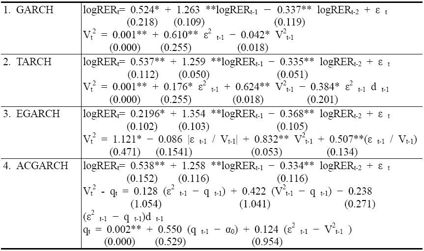
The pure GARCH model and three asymmetric GARCH models have been estimated systematically. The results of the estimation using won/dollar real exchange rates are shown in Table 1, and those for won/yen are shown in Table 2. In terms of the won/dollar exchange rate, significant ARCH and GARCH effects appear to exist in the data: the coefficients in both the mean and variance equations of the real exchange rates are significantly different from zero. In addition, asymmetric GARCH models are empirically successful. Of these models, the TARCH and EGARCH models are effective in modeling asymmetric effects, providing statistical evidence consistent with the asymmetric effect. Specifically, the coefficient for the asymmetric effect in TARCH is -0.384 and statistically significant at the 5 % level, and the coefficient in the EGARCH model is 0.507 statistically significant at the 1 % level.
The estimation using won/yen real exchange rates provides similar results. Significant ARCH and GARCH effects appear to exist in the data as the coefficients in both the mean and variance equations of the real exchange rates are statistically different from zero. Of these models, the TARCH and EGARCH are effective in modeling asymmetric effects, providing statistical evidence that is consistent with the asymmetric effect. Specifically, the coefficient for the asymmetric effects in TARCH is -0.606 and statistically significant at the 5 % level. The coefficient in the EGARCH model is 0.45 and statistically significant at the 5 % level.
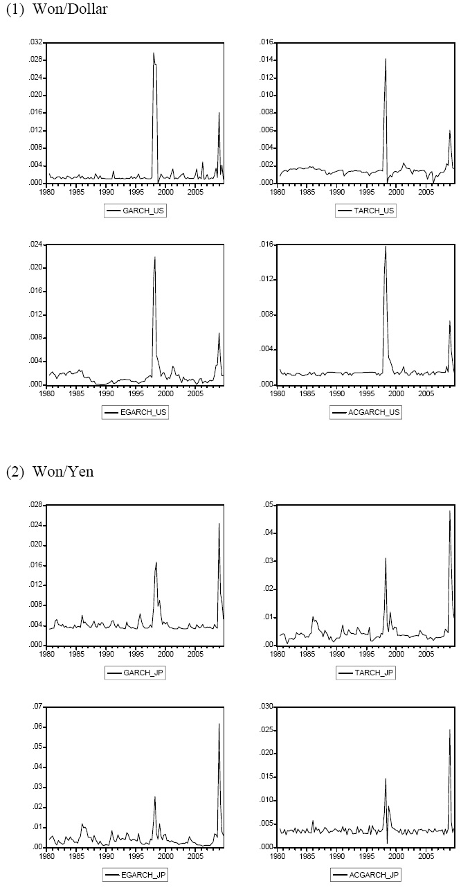
Asymmetric effects in conditional variance asymmetry from the results may be due to market participants’ predictions of the variance in the current period’s real exchange rates, which has been suggested by Black (1976). This variance is measured as the weighted average of the long-term average and the ARCH and GARCH/ asymmetric GARCH terms. Thus, the predicted values of the conditional variance from the asymmetric GARCH specifications provide a better measure of the exchange rate volatility of the Korean won against the U.S. dollar and the Japanese yen. The predicted values are used as exchange rate risks in estimating the exports equation. Figure 1 presents graphical representations of the volatility of the won/dollar and won/yen exchange rates.
[Table 1] Estimation of the Won/Dollar Real Exchange Rate (1980:Q1~2009:Q4)

Estimation of the Won/Dollar Real Exchange Rate (1980:Q1~2009:Q4)
[Table 2] Estimation of the Won/Yen Real Exchange Rate (1980:Q1~2009:Q4)
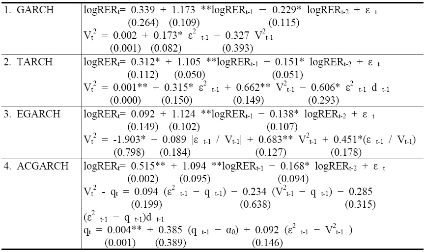
Estimation of the Won/Yen Real Exchange Rate (1980:Q1~2009:Q4)
As discussed earlier, to examine the time-series properties of individual series, a preliminary procedure for the stationarity property of the concerned variables is followed using the augmented Dickey- Fuller (ADF) unit root test. The results are shown in Table 3. The optimal lags for the ADF test are chosen with the Schwarz information criterion (SIC). They indicate that all the variables (except for the conditional variance) are non-stationary at their level, and the series at the first difference are stationary. These results are consistent with the recent findings of Anderson et al. (2001) and Klaasen (2004), who showed that exports, real foreign income, and real exchange rates typically have unit roots. On the other hand, the conditional variance in exchange rate is found to be stationary. If all concerned variables are nonstationary and integrated of the same order, it takes a conventional procedure to investigate the possibility of uncovering useful cointegrating relationships that can form the basis of estimating an error correction model (ECM). Such cointegrating relationships can specify the dynamics in a manner that forces the short-run relationships to be consistent with their long-run counterparts. For there to be a cointegrating relationship between these variables, each series should be a unit root and integrated of the same order (Engle and Granger, 1987). The results from the ADF tests in Table 3, however, indicate that these variables are integrated of different orders; exports, real foreign income, and the real export price are I(1) and, on the other hand, the conditional variance is I(0). These results rule out the examination of a useful cointegrating relationship and the ECM representation of the data generation process in the present research (Engle and Granger, 1987). Instead, as discussed earlier, the bounds testing approach to cointegration advanced by Pesaran, et al (2001) is applied to test the asymmetry hypothesis. This technique has an interesting property in that there is no need for the same order of integration. In other words, the bounds testing approach is free from the order of integration. Thus, this approach is suitable to the present study because whereas the volatility measure of the bilateral exchange rate may be stationary, other variables such as exports and income may be non-stationary. The next section presents the results of the estimation of the export equations by using the unrestricted error-correction model (UECM) format that follows the bounds testing approach explained above.
[Table 3] Augmented Dickey-Fuller (ADF) Statistics for the Unit Root Tests
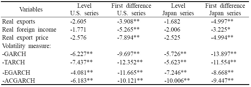
Augmented Dickey-Fuller (ADF) Statistics for the Unit Root Tests
3. Estimation results for bounds testing
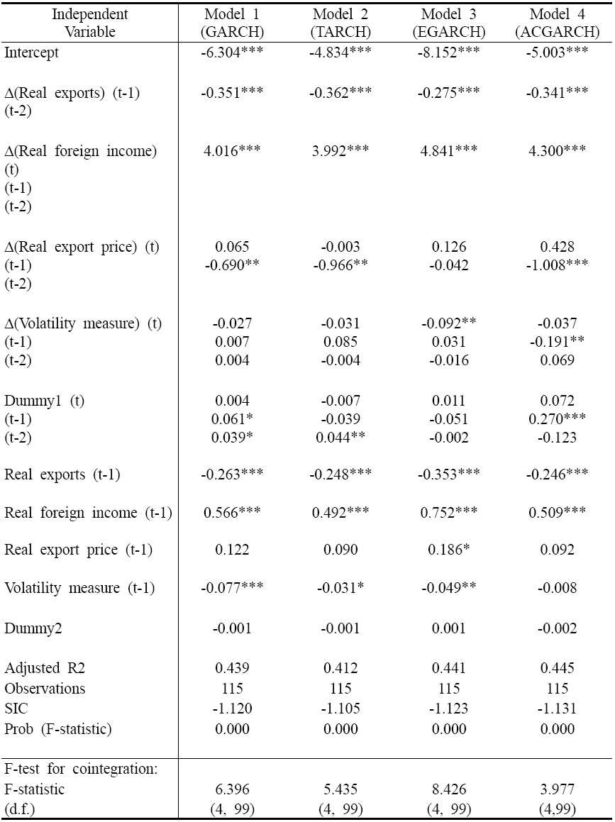
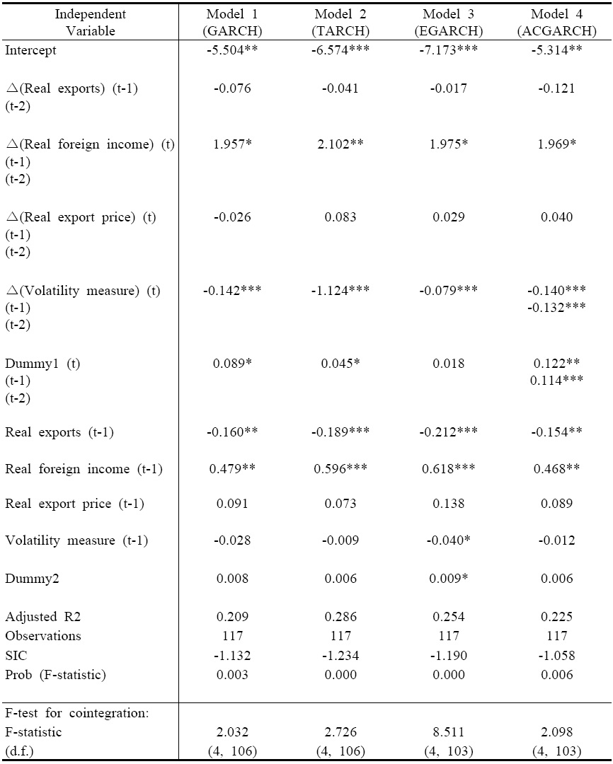
Tables 4 and 5 present the estimation results for the bounds testing specification of the export demand equation (4) from Korea to the U.S. and to Japan, respectively. The optimal lags for the bounds testing estimation are chosen with the Schwarz information criterion (SIC). The column “Model 1” shows the result for the case in which the predicted value of the conditional variance from the GARCH specification is used as a proxy for exchange rate risk. The column “Model 2” shows the results for the case in which the TARCH measure is used, the column “Model 3” for EGARCH, and the column “Model 4” for ACGARCH, respectively. In addition, the last row reports the F-statistic for the long-run cointegrating relationship between the variables, which is obtained by taking the bounds testing approach specified in Equation (4). According to the test statistics, all of the four cases for the U.S. support strong cointegration relations at the 1% level of significance, but the results for the two cases for Japan are significant at the 1% and 5% levels. As expected, the results for the long-run cointegration relations indicate that an increase in the real GDP of the U.S. (or Japan) is likely to result in an increase in Korean exports to the U.S. (or Japan) in the long-run. On the other hand, in the short-run, the income effect is found to be more significant and stronger for the U.S. market than that for the Japanese market. Further, the price effect is found to be significant only for the U.S.
1) Dynamic effects
As for the focus of the study that is to evaluate the short-and long-run dynamic effects of exchange-rate volatility, there are some noteworthy results. As shown in Tables 4 and 5, the results provide support for the hypothesis that an increase in exchange rate volatility results in a decrease in export volume. Exchange rate risk has significant effects on exports to the U.S. and Japan; the effects are negative when exchange rate is depreciating and positive when it is appreciating. However, the dynamic of the uncertainty effects varies according to the trading partners. According to the estimation of the four estimates of the volatility measures, the short-run negative effect is dominant for Korean exports to the Japanese market. All the volatility coefficients in Table 5 are found to be negative and significant at the 1 % significance level, and there is no significant evidence for the long-run effect of exchange rate volatility (except for Model 3). On the other hand, whereas the long-run effect for the U.S. is significant, the coefficient estimates for volatility in the short-run are found to be statistical significant for all of the four models for Japan, and for two of the models for the U.S.
2) Asymmetric effects
The short-run asymmetric effects as well as the long-run asymmetric effects of exchange rate volatility are examined. First, according to the estimated coefficients of the dummy variable for the long-run cointegrating relation (Table 4 and 5), there is no significant evidence for the long-run asymmetric effect. As shown in Table 4 and 5, there is no significant evidence to be found for both the U.S. and Japanese markets.
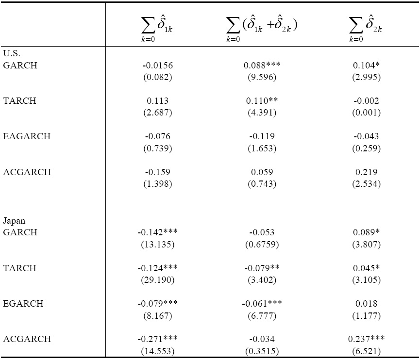
Next, Table 6 shows the results of the sum tests for the short-run asymmetric effect of exchange rate volatility. The likelihood ratio (LR) statistic with an
that is, whether the total influence of exchange rate risk on exports equals zero for depreciation, for appreciation, or for the differences between two sums. The coefficient sums of exchange rate risk during the depreciations of the exchange rate significantly differ from zero and negative effects for all four models in Japan. The magnitude of the sum ranges from -0.079 in the EGARCH model to -0.271 in the ACGARCH model. The coefficient sums during appreciation significantly differ zero for the TARCH and EGARCH models. The two models exhibit a significantly negative sum. The magnitude ranges from -0.061 to -0.079. By contrast, the test statistics provide inconclusive results for Korean exports to the U.S. market. They exhibit a mixed negative, less negative or positive effect during depreciations or appreciations for the GARCH and TARCH models. There is no statistically significant evidence that the coefficient sums of exchange rate risk in depreciation are significantly different from zero for all four models for the U.S. The coefficient sums during appreciation significantly differ from zero for the GARCH and TARCH models. These two models exhibit a significantly positive sum. Estimates are 0.088 and 0.110 at the 1 % and 5 % significant levels. However, the estimates should be interpreted with caution since the magnitude of estimates includes instantaneous and lagged effects of the volatility on Korean exports to the U.S. Market. This magnitude should be interpreted together with the results for the short run effect on exports to the U.S. in Table 4. Bounds testing estimation for Korea-US in Table 4 shows that the volatility has both an instantaneous and lagged effect on exports to the U.S.; in particular, there is an instantaneously negative effect and some lagged positive effects. Thus, the total magnitude for the U.S. in Table 6 could be positive, since the lagged positive effect might dominate the instantaneous negative effect. In other words, the result in Table 4 and Table 6 implies that the volatility of the exchange rate may have an instantaneously negative effect on Korean exports to the U.S. market, but have positive effect with lags. In fact, the finding for the positive effect in Korean exports to the U.S. is consistent with the arguments and findings for a positive hypothesis in previous studies such as Franke (1991), Dallas and Zilberfarb (1993), Mckenzie and Brooks (1997) and Mckenzie (1998).3 They show the evidence for a significantly positive effect of exchange rate volatility on U.S.-German and U.S.-Australian bilateral trade, and suggest that the direction as well as the magnitude of the impact of volatility may differ according to trading markets. In sum, these results support the argument that Korean exporters respond differently to exchange rate risk in periods of depreciation and appreciation of exchange rates because of currency mismatches in exports. However, the effect varies according to the individual trading partners (i.e., the U.S. and Japan in this study).
Estimations further show tests for the second form of significant asymmetric effects. Because the exchange rate risk proves significant on exports either in depreciation or appreciation, the difference between the two coefficient sums determines the test. The difference sums of

for Japan are significantly different from zero and indicate different magnitudes for the depreciation and appreciation risk affects. Three models for Japan exhibit a significant asymmetric effect. Positive risk effects in difference sums appear ranging from 0.089 to 0.237 (Table 6) for Japan. This implies that Korean exporters targeting the Japanese market could aggressively manage the adverse effects of appreciating exchange rates to achieve a less negative effect, but leave the beneficial effects of depreciation not managed. On the other hand, the test results for the U.S. show no significant evidence for the asymmetric effect in the short-run for Korean exports to the U.S. market, indicating that Korean exporters targeting the U.S. market are unlikely to behave asymmetrically to the asymmetric response. This finding raises the question of whether different export markets affect exchange rate risk differently when the exchange rate depreciates or appreciates.
In general, the results of this paper support the idea that exchange rate risk affects exports asymmetrically. However, the results suggest that the asymmetric effect varies according to the export market. This response asymmetry may arise from a variety of sources such as asymmetric risk perception, fear of an appreciating exchange rate, and pricing-to-market behavior, which in-volves adjusting export prices based on the degree of competition in specific foreign markets. The mixed results for the dynamics of asymmetric effects for the U.S. and Japan may be due to differences in a trader’s response to sources. For example, this asymmetric effect may occur as a result of possible differences between Korean exporters’ pricing-to-market behaviors for the U.S. market and that for the Japanese markets, which is consistent with the findings of Marston (1990) and Goldberg (1995)4, who examined the market share objective and asymmetric characteristics between countries and found asymmetric pricing-to-market behavior and its difference in destined export countries.
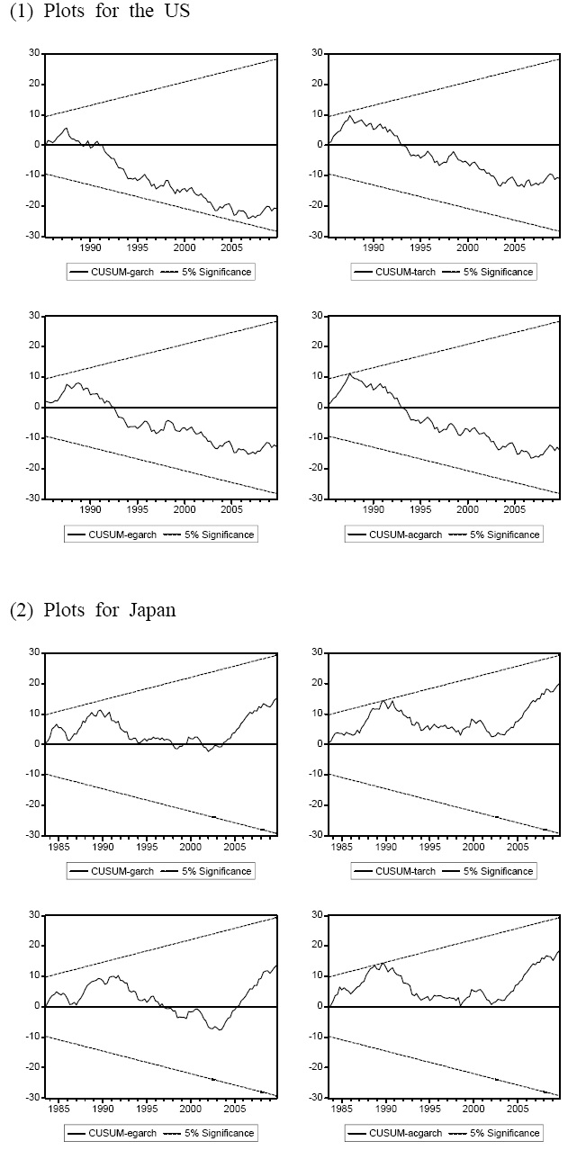
3) Stability tests
Finally, to investigate the stability of the estimation and the coefficient estimates, the procedure for the stability test is followed using the Cumulative Sum (CUSUM) test (Brown et al., 1975). The CUSUM statistic is based on the cumulative sum of the recursive residuals to examine whether the parameters of the model are stable across various sub-samples of the data during the sample period. Test results are shown in Figure 2. It plots the cumulative sum together with the 5% critical lines. The test finds parameter instability if the cumulative sum goes outside the area between the two critical lines. The figures clearly indicate the absence of any instability of the coefficients in the estimation for all cases of the U.S. and Japan during the sample period, because the plot of the CUSUM statistic is confined within the 5% critical bounds of parameter stability.
3In particular, Franke (1991) analyzed the export strategy of a risk neutral firm operating in a monopolistic competition framework and provided support for the positive hypothesis. 4Marston (1990) examined the pricing-to-market behavior of Japanese manufacturers, and Goldberg (1995) focused on the automobile industry.
This study examines whether exchange-rate volatility can lead to decreases in Korean exports to the U.S. and Japan. The results of the bounds testing estimation based on the unrestricted error correction model indicate that the dynamic effect of exchange rate volatility and its asymmetry differ with respect to the individual trading partner. The results provide statistically weak evidence of the long-run equilibrium cointegration relationships among the variables of the real exports demand function for Japan, but strong evidence for the U.S. The results for Japan support evidence for the short-run adverse effect of exchange rate volatility on exports, whereas those for the U.S. provide evidence for the long-run negative effect. Furthermore, the short-run estimation results for the unrestricted error correction model are consistent with the results for the long-run parameter estimates. Further, the asymmetric effect varies according to both the trading partner and the volatility specification. There are short-run asymmetric effects for Korean exports to Japan, but there is no strong evidence supporting the short-run asymmetry hypothesis for the U.S. The empirical findings of this paper support the conclusions of previous studies (e.g., Mckenzie and Brooks, 1997; Mckenzie, 1998; Onafowora and Owoye, 2008).
In addition, the present study provides more specific and detailed evidences for the dynamic effect of the asymmetry. Previous empirical studies have typically examined the effects of exchange rate risk without differentiating the asymmetric responses. The present study’s model of the asymmetric and dynamic effects provides a better understanding of the effect of exchange rate uncertainty on a country’s exports than the models of the symmetric effect used in previous studies. The findings suggest that policy makers should consider the stability of the exchange rate, trading partners, and dynamics of the exchange rate during its appreciations and depreciations when managing export movements. In particular, the asymmetric risk effects have an important implication for policy makers. Conventionally, it is argued that a depreciating exchange rate increases exports, but the exchange rate uncertainty induced by the depreciation can hurt exports. Thus, the existence of asymmetric effects and the difference in the effects according to the trading partner may further complicate and increase the uncertainty over trade policy. Thus, any successful trade policy requires a full understanding of the dynamics of exchange rate risk as well as a careful consideration of its asymmetry and the trading market. This study suggests that policy makers need to be cautious in intervention of the foreign exchange market in order to increase exports and improve the trade balance, but rather they should understand the movement of exchange rate uncertainty, paying particular attention to the stability of the exchange rate (e.g., smoothing operation for lessening exchange rate volatility), and consider a differentiation trade policy according to the trading market.
[Table 4] Bounds Testing Estimation of the Export Function (Korea-US)

Bounds Testing Estimation of the Export Function (Korea-US)
[Table 5] Bounds Testing Estimation of the Export Function (Korea-Japan)

Bounds Testing Estimation of the Export Function (Korea-Japan)
[Table 6] Tests for the Short-run Asymmetric Effect of Exchange Rate Risk

Tests for the Short-run Asymmetric Effect of Exchange Rate Risk
This study cannot be considered complete and consistent in its current form. The conclusions of this paper await further refinement and correction in the light of further research. This paper concerns itself with the existence, rather than the sources, of the asymmetry. Future research can consider the specific sources of the asymmetric effects to provide a better understanding of the role of exchange rate volatility and its asymmetry.