Because an ecological community consists of diverse species that vary nonlinearly with environmental variability, its dynamics are complex and difficult to analyze. To investigate temporal variations of benthic macroinvertebrate community, we used the community data that were collected at the sampling site in Baenae Stream near Busan, Korea, which is a clean stream with minimum pollution, from July 2006 to July 2013. First, we used a self-organizing map (SOM) to heuristically derive the states that characterizes the biotic condition of the benthic macroinvertebrate communities in forms of time series data. Next, we applied the hidden Markov model (HMM) to fine-tune the states objectively and to obtain the transition probabilities between the states and the emission probabilities that show the connection of the states with observable events such as the number of species, the diversity measured by Shannon entropy, and the biological water quality index (BMWP). While the number of species apparently addressed the state of the community, the diversity reflected the state changes after the HMM training along with seasonal variations in cyclic manners. The BMWP showed clear characterization of events that correspond to the different states based on the emission probabilities. The environmental factors such as temperature and precipitation also indicated the seasonal and cyclic changes according to the HMM. Though the usage of the HMM alone can guarantee the convergence of the training or the precision of the derived states based on field data in this study, the derivation of the states by the SOM that followed the fine-tuning by the HMM well elucidated the states of the community and could serve as an alternative reference system to reveal the ecological structures in stream communities.
Ecological processes are not easily observable due to the complexity in responding to numerous environmental conditions. In many cases of ecological research, observed patterns are considered as the result of underlying ecological states embedded in complex ecological processes with different governing rules than simple consequences of the observations. The data are also highly variable due to noise, and redundancy, internal relations and outliers are often observed (Gauch 1982, Jongman et al. 1995). Conventional indices such as Bray-Curtis similarity have been proposed to reveal the temporal dynamics of stream community (Scarsbrook 2002, Collier 2008). In addition multivariate analyses also have been applied to extraction of high dimensional temporal data to obtain ecological integrity in reduced dimension (Legendre and Legendre 1998, Scarsbrook 2002, Beche and Resh 2007). For the former method, however, the parameters are constrained in a sense that community dynamics is only expressed by a single term, whereas the latter method could reveal statistical or overall patterns in complex data, being insufficient in addressing ecological processes objectively.
Markov processes were suitable in addressing complex time series changes depending on time, location, and local or global state frequency (e.g., characterizing clean or pollution states) (Tucker and Anand 2003) in plant (Horn 1975, Yemshanov and Perera 2002) and animal (Usher 1981, Hill et al. 2004) ecology. Markov models that implement Markov processes have been developed in two different manners: a stationary Markov model (SMM) and a hidden Markov model (HMM). Since 1960 (Baum and Petrie 1966, Baum 1972), the HMMs have arisen for overcoming the limitation of the SMM (monotonic increases or decreases), because they are more adaptable to complex situations (Rabiner 1989, Visser et al. 2002). The HMMs are described as “hidden” because the sequence of observation events (e.g., sequences of ecological data) is the result of a stochastic process operating on top of a sequence of hidden states generated by a Markov process (Rabiner 1989). Based on stochastic processes applied to observable events and states concurrently, the discrete states are more clearly addressed in the HMM than in the SMM.
The HMM could be suitably applied to ecological processes and allows the description of the complexity including interacting hierarchical systems and hidden processes underlying the observed ecological dynamics (Tucker and Anand 2004). HMMs are also flexible and relatively easy to implement because efficient algorithms have been developed to estimate the model parameters (Ghahramani and Jordan 1997). The HMM has been feasible for analyzing animal behaviors (MacDonald and Raubenheimer 1995, Liu et al. 2011), and the wide biological disciplines including DNA and protein sequencing analysis (Krogh et al. 1994, Karplus et al. 1997). Although HMMs have been widely applied to ecology, there have only been a few attempts to analyze community dynamics, especially for benthic macroinvertebrates in streams. The HMM was utilized to address vegetation community dynamics in remote sensing (Viovy and Saint 1994), change-points in grassland vegetation (Ver Hoef and Cressie 1997), and coastal wetland processes (Dale et al. 2002).
Prior to applying the HMM, the candidates for states were obtained heuristically by applying a self-organizing map (SOM) to the field data in this study. Based on SOM clustering, transition probabilities were estimated between states according to varying time series data. The SOM is an unsupervised neural network and has been implemented in various ecological studies (Adriaenssens et al. 2007, Chon 2011). The SOM has been a feasible means to address changes in temporal patterns (Voegtlin and Dominey 2001, Simon et al. 2007) including benthic macroinvertebrates (Chon et al. 2000) and fishes (Hyun et al. 2005).
The current study is aimed to finely define the states in temporal dynamics of benthic macroinvertebrate communities with minimum pollution by the HMM based on the initial data heuristically obtained from the SOM. Based on taxonomic diversities, sedentariness in survival range, and long life cycles, benthic macroinvertebrates characteristically respond to the changes of environment from watershed areas (Resh and Rosenberg 1984, Park et al. 2007, Tang et al. 2010). Although the community of benthic macroinvertebrates presents ecological integrity fairly well, community data are highly complex and difficult to analyze because communities consist of numerous species varying in a complex and stochastic manner in response to environmental factors (e.g., high precipitation) in monsoon areas in East Asia (Chon et al. 2001).
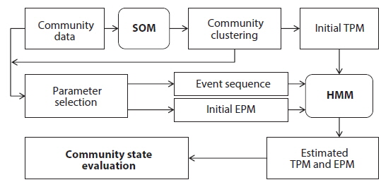
In this study, we hypothesized that the temporal changes of the community could be stably expressed in the natural stream environment of monsoon areas. Partial information on community states based on field data was obtained by the SOM to provide an initial transition probability matrix (TPMs) and emission probability matrix (EPMs) for the HMM. Subsequently, the HMM was conducted according to the observable event sequences including biological (e.g., number of species and diversity) and environmental (temperature and precipitation) parameters. Community states preserved in benthic macroinvertebrates in streams were addressed accordingly by responding to natural variability to present structure property residing in community changes more objectively.
The Nakdong River is the longest river flowing through the Busan-Daegu Metropolitan areas in the southern part of the Korean peninsula. A sampling site, BCN (coordinates, 35°31′07.72″ N, 128°01′01.97″ E; altitude, 398 m), located in the Baenae Stream, a tributary of the Nakdong River, in the mountainous area near Busan (Tang et al. 2010) was selected for the study. BCN is considered as a reference stream with the minimal environmental impact (BOD, 1.1 mg/L; conductivity, 24.6 μS/cm) for the national Long-Term Ecological Research (LTER) project in Korea. Since 2005, BCN has been a sample site for LTER supported by the Korea’s Ministry of Environment.
Sampling was conducted monthly by the Surber sampler (30 × 30 cm, 100 μm mesh) in 5 replications at a sampling site from July 2006 to July 2013. The environmental factors such as temperature and conductivity at sampling site were additionally measured (Table 1) by YSI 30 conductivity-salinity meter (Yellow Springs Instruments, Yellow Springs, OH, USA). The specimens were mostly identified to species or to the lowest possible taxonomical level by following the procedure described by Merritt and Cummins (1996), Brigham et al. (1982), Pennak (1978) and Yoon (1995) for general taxa, Brigham et al. (1982) and Brinkhurst (1986) for Oligochaeta, and Wiggins (1996) for Trichoptera. Chironomidae, however, was not identified at the species level due to the difficulty of classification. After classification of the specimens, species diversity was determined according to the Shannon index (Shannon and Weaver 1949). Biological indices, the number of species in EPT (Ephemeroptera, Plecoptera, and Trichoptera) taxa, biological monitoring working party (BMWP) and average score per taxon (ASPT) (Hawkes 1998), were also obtained to assess the water quality. The average and standard error of parameters in different seasons were presented in Table 1.
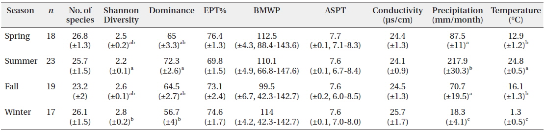
Biological indices and environmental parameters, represented as mean (±SE), at BCN in different seasons
In the SOM network, the output layer consisted of computation nodes (

In this study the data matrix for the SOM consisted of 77 sample units (monthly collection from July 2006 to July 2013) and 69 variables (total number of species collected during the survey period). In order to reduce the great difference of numerical values in densities for SOM training, the input data, i.e., densities (individual/m2) plus one individual, were transformed by common logarithm.
After training, the Ward’s linkage method (Ward 1963) was applied to the weights of the SOM to cluster the patterned nodes. The initialization and training processes followed suggestions by the SOM Toolbox to allow optimization in algorithm (Vesanto et al. 2000). To evaluate the map quality, the quantization error for the resolution and the topographical error for the topology preservation were used to indicate the accuracy of mapping (Céréghino and Park 2008, Kohonen 2001, Park et al. 2003). More details in training and clustering were performed according to Park et al. (2003) under the MATLAB 6.1 environment (The Mathworks, Inc., Natick, MA, USA).
Markov chain calculates the transition probabilities between community states from one time step to the next (Wootton 2001b, Tuker and Anand 2004). When the system has a finite set of discrete states (the number of states was estimated by SOM), these transition probabilities can be presented in a transition probability matrix where

An HMM can be characterized by five elements (Rabiner 1989):
(1) A number of states N, x ∈ {1, . . ., N}; (2) A number of events K, k ∈ {1,. . ., K}; (3) Initial state probabilities, π = { πi} = {P(x1 = i)} for 1 ≤ i ≤ N; (4) State-transition probabilities, A = {aij} = {P(xt = j | xt−1 = i)} for 1 ≤ i, j ≤ N; (5) Discrete output probabilities, B = {bi(k)} = {P(ot = k | xt = i)} for 1 ≤ i ≤ N and 1 ≤ k ≤ K,
where in (5),
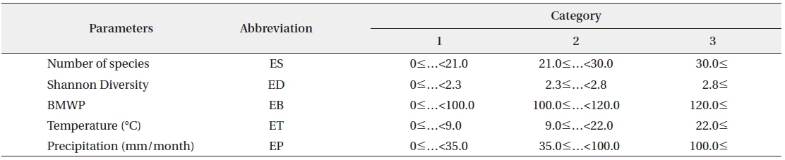
The transition probability matrix according to the SOM was used as initial TPM for HMM (Fig. 1). Transition probabilities across different states based on the SOM were accumulated and average transition probabilities between different community states were obtained. Subsequently we selected the biological indices (number of species, diversity and BMWP) and environmental factors (temperature and precipitation) as the observation events, because these parameters could represent the states of community with simple measurements (Fig. 1). Each parameter was divided into three levels based on the difference in SOM clustering analysis. Then three levels were considered as different categories defining each event (Table 2). Temporal dynamics of each event in the monthly scale were considered as event sequences. The initial EPM for HMM was further obtained by calculating probabilities of events corresponding to states given by the SOM in time series data.
[Table 2.] Category of biological and environmental parameters in three levels

Category of biological and environmental parameters in three levels
Initial TPMs, EPMs and event sequences were also given to HMM as input data for training. Subsequently TPM and EPM were estimated according to the Baum-Welch algorithm for each event parameter (Juang and Rabiner 1991, Rabiner 1989, Durbin et al. 1998) (Fig. 1). The algorithm halted when the matrices in two successive iterations were within a tolerance value (0.1) for the discrete HMM (Taheri et al. 2005). If the algorithm failed to reach this tolerance within a maximum number of iterations, the default value for termination was 100 iterations. Based on the solutions presented in Rabiner (1989), the process was conducted with the programs provided in the HMM toolbox in MATLAB 2009 (The Mathworks, Inc.).
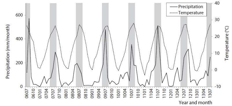
While sampling the community data, we also recorded monthly changes in precipitation and temperature as presented in Fig. 2. Those environmental factors varied at the sampling site according to the seasonal monsoon climate in Korea: high temperature (24.8℃) and precipitation (217.9 mm/month) in summer, and low temperature (1.3℃) and rainfall (18.3 mm/month) in winter (Fig. 2 and Table 1). The environmental factors showed distinct and unique features in summer and winter, while those in spring and fall were somewhat similar. Diversity was substantially low with high dominance in the summer. Biological water quality indices, however, EPT% (the percent EPT species in community), BMWP and ASPT, were relatively constant in seasonal changes (Table 1).
>
Patterning by the self-organizing map
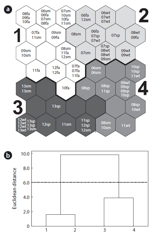
To reveal patterns underlying the community data, we initially analyzed the monthly data of community abundance by training the SOM (Fig. 3a). In Fig. 3b, the clusters were divided into two distinct groups on the SOM based on the Ward’s linkage method: two clusters of 1 and 2 in the upper part and other two clusters of 3 and 4 in the bottom part of the map. Cluster 1 contained the majority samples in summer and fall samples (Fig. 3a). In cluster 2, winter samples dominated. Spring and some other winter samples were spread over all parts of the SOM, with a weak bias toward the bottom part of the SOM (clusters 3 and 4).
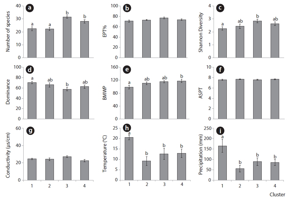
Fig. 4 shows the average values of biological indices and environmental parameters for each cluster. The number of species was significantly high in clusters 3 and 4 in the lower area of the SOM along the vertical gradient (Fig. 4a) (ANOVA,
In particular, the environmental factors could characterize each area in the SOM. Temperature and precipitation were significantly high in cluster 1 consisting of the community data in summer and fall on the upper group of the SOM (Fig. 4h and 4i). Communities in cluster 2 presented low precipitation and temperature that characterized winter samples although statistical significance was not shown here. Conductivities were invariably low across clusters (Fig. 4g). Overall, communities in cluster 1 that were characterized with low diversity were influenced by high precipitation and temperatures, whereas communities in cluster 3 that were featured with high diversity and low dominance were affected by mid precipitation and temperatures.
>
Initial transition probability matrix
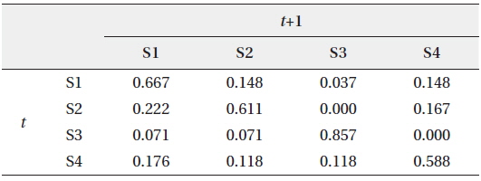
We hypothesized that patterns of the community data clustered by SOM (i.e., extraction from field data) could be useful to provide initial information for estimating the states of the community. These patterns could be provided to HMM as initial state transition probabilities, assuming that the clusters derived by the SOM training could represent the states of community in the field condition accordingly (Fig. 1). After SOM recognition, the probabilities to transit from one state (cluster) to the other state (cluster) were computed from the time series data. The obtained initial TPM is shown in Table 3. High remaining probabilities in the same states were observed for all the states (diagonal elements in Table 3) and it confirmed the robustness of probabilities. State 3 (S3) showed the highest remaining probability (0.857) whereas relatively low remaining probability was observed in state 4 (S4), showing 0.588. The probabilities transiting between different states have low values that ranged from 0.1 to 0.2. It was noteworthy that the S3 showed exceptionally low transition probabilities less than 0.1 except transition from S3 to S3 (S4→S3). Asymmetric transition probabilities were observed in relation to S3, for instance S3→S2 (0.072) and S4→S3 (0.118) (Table 3).

Initial transition probability matrix (TPM) between different states (S) at time t and t+1 according to the self-organizing map (SOM)
>
Estimated transition probability matrices and emission probability matrices
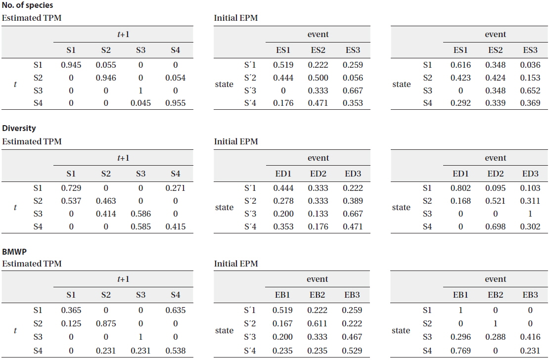
The biological parameters presenting the structure of the community (the number of species and the diversity) and the water quality (BMWP) were also obtained from the community data as observable events for HMM (see the “Hidden Markov model” section in Materials and Methods) (Table 2). The time series data were used as input event sequence to train the HMM. We also categorized each event depending on its value (i.e., low, medium, and high) (Table 2). The emission probability matrix (EPM) was determined by calculating the probabilities of all the events assigned to each state in time series data (Fig. 1). The initial EPM is shown in Table 4 for the selected parameters, the number of species, the diversity, and the BMWP. The TPMs and the EPMs were accordingly estimated through the HMM (Fig. 1) for different event variables (Rabiner 1989) (Table 4). The sum of probabilities for each matrix was normalized to unity; the sum of the probabilities in each row was set to 1.0 in total. Initial and estimated TPMs for three events were statistically not different (Table 4) based on the Kolmogorov-Smirnov tests (Quach et al. 2013) (
[Table 4.] Estimated TPMs and initial and estimated EPMs for biological and environmental parameters

Estimated TPMs and initial and estimated EPMs for biological and environmental parameters
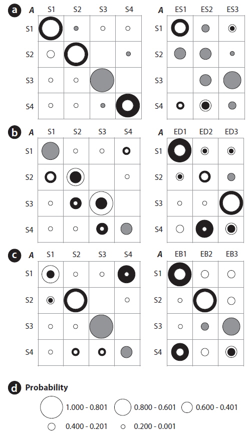
The estimated TPMs for the number of species had a strong tendency to show high probabilities to remain in the same state (Table 4). All probabilities in the diagonal elements were close to unity, ranging from 0.945 to 1.000. The estimated probability to remain in S4 remarkably increased to 0.955 from the initial transition probability of 0.588 (Table 3 and 4). The estimated EPM also characterized well the states of the community that were determined by the SOM (Table 4). In state 1, the frequency of low species number increased, ES1 (0.616). This indicated that state 1 comparatively depicted the stressful conditions of communities with low species number. State 3 showed the highest frequency with high species number, ES3 (0.652). Other states of 2 and 4 were characterized by mixed categories showing evenly high probability with low and/or intermediate species number for state 2, and evenly high probability with intermediate and/or high species number for state 4 (Table 4). The event characterization according to estimated EPMs for different states was also in accordance with the results from the SOM and field experience (Fig. 4).
The estimated transition probability for the diversity appeared lower diagonal elements than that for the number of species (Table 4). The probabilities for S2→S1 (0.537) and S4→S3 (0.585) were higher than those to remain in the same states S2 (0.463) and S4 (0.415), respectively. The estimated EPM could also characterize the community states (Table 4). In general, the emission probabilities seemed similar to the number of species. However, event categories were more strongly correlated with the states. State 1 corresponded to low diversity, ED1 (0.802), with high emission probability. The highest emission probability of 1.0 was associated with high diversity, ED3, at state 3. The emission probabilities corresponding to the diversity were differentiated more clearly (i.e., larger distance between maximum and minimum probabilities) than the number of species (Table 4). The estimated TPMs based on the BMWP showed the states were reluctant to remain in the same states except S3 (1.0) and had tendency of transition to other states more, especially S1→S4 (0.635) (Table 4). The estimated emission probabilities, however, were well separated, including 1.0 for the case of S1:EB1 and S2:EB2. Comparing with the estimated EPM, state 3 presented higher tendency to the high BMWP (EB3) than state 4.
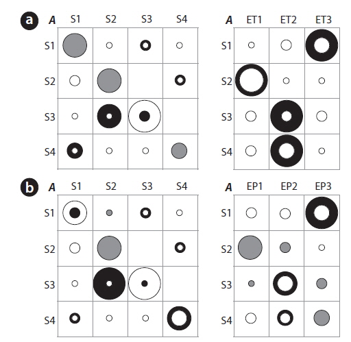
Differences between the initial and the estimated values of the TPMs (left panel) and the EPMs (right panel) are further shown in Fig. 5a-5c. Training with the number of species substantially increased the probabilities to remain in the same states (i.e., the thick black rings in Fig. 5a). The diversity, however, resulted in the substantial reduction in the probabilities to remain in the same states (i.e., the white rings in Fig. 5b). For the transition probabilities to other states (the off-diagonal elements in the TPMs), only the diversity showed distinct changes with cyclic pattern. Consequently it can be conjectured that the probabilities of state changes were more strongly expressed with diversity whereas discreteness in self-transition probabilities were more clearly addressed in the case of the number of species (Fig. 5). The EPMs also accordingly characterized the states as shown in Figure 5. Regarding the number of species, state 3 matched high number of species (ES3) whereas state 1 corresponded to low number of species (ES1). States 2 and 4 showed a mixed abundance of lowintermediate (ES1, ES2) and intermediate-high (ES2, ES3) levels of the number of species, respectively. For the diversity, the estimated probabilities substantially increased for S1:ED1, S3:ED3, and especially S4:ED2 (Fig. 5b). It means that the states of 1, 4 and 3 were likely to have the low (ED1), the middle (ED2) and the high diversity (ED3), respectively. State 2 was evenly associated with intermediate and high diversity (Fig. 5b), and was considered as a connection between two states S1 (low diversity) and S3 (high diversity).
We further checked if the water quality data that was empirically measured (i.e., BMWP) could preserve the transition probabilities based on the HMM training (Fig. 5c). A substantial change was observed regarding S1 in the estimated TPM. Probability for S1→S4 was markedly increased, and transition probabilities regarding S4→S3, S4→S2 and S2→S1, were also observed although the values were relatively low in TPM for BMWP. State 4 tended to be both state 2 (the middle value of BMWP) and state 3 (the high value of BMWP), and it indicated that state 4 was a link between the states of the low and high BMWP. The estimated EPM based on BMWP showed a similar trend to the case of the diversity. The maximum emission probabilities clearly appeared in all states, which showed the distinct association between the water quality and the states of the community (Fig. 5c). For instance, state 1 showed higher emission probability to the low BMWP than to the low diversity. However, state 2 was exceptionally characterized by the middle value of BMWP at EB2 whereas middle value of the diversity was shown at state 4 with ED2 (Fig. 5). Consequently, the EPM elaborated by training with the BMWP was more clearly characterized with high frequency of EB1, EB2 and EB3 for S1, S2 and S3, respectively. S4 was split in matching two event categories, EB1 followed by EB3. This demonstrated that the empirically determined BMWP could complement changes of community state that were partially observed in fields. The overall results suggested that the diverse aspects in states could be revealed according to different biological parameters.
To diagnose the integrity and the healthy condition of the communities from the field data, we developed a novel method to indicate the temporal states of communities by combining two computational methods of the SOM and HMM. By using the heuristic SOM as input data, stochastic processes residing in community development processes were accordingly elucidated to demonstrate a structure property of community. In most studies, the initial transition probabilities were given as either uniform or random distribution to train the HMM by assuming that the states were totally unknown. However, this approach does not guarantee to achieve the convergence to obtain the estimated TPMs in this study. It was mainly originated by the short and partial sequences of the field data (77 sequences for monthly sampling in this study). This study demonstrated how to combine the short information obtained from field data by applying the SOM and the HMM consecutively to address ecological processes observed in benthic macroinvertebrate in field condition in depth. First, by clustering the SOM, we could combine many pieces of information that describe the different aspects of the community and derive the state of the community. Second, by applying the HMM, we could find the impact of the different pieces of information on each state objectively and the strong consistency among different parameters as well (Fig. 1). We also showed that the inferred time series data of the states could depict the seasonal dynamics of the community in detail (Figs. 4 and 5).
This paper showed that the different aspects of the community states could be concurrently measured and analyzed with respect to different observable events such as the number of species, the diversity, and the BMWP. While the number of species was distinctively specialized in defining states (discreteness in community states from the high diagonal elements in TPM), the diversity showed the cyclic development of communities (Fig. 5 and Table 4). Remarkably, the estimated TPM derived by the diversity could efficiently address the seasonal changes of states. According to the temperature for each state shown in Figure 4h based on the SOM, we could find that state 1 and 2 represent the summer and winter seasons, respectively. The development of community with cyclic pattern were presented, S1 (the low diversity in summer)→S4 (the variable diversity in transition)→S3 (the highest diversity in transition)→S2 (the variable diversity in winter)→S1 (Fig. 5b and Table 4). Two states of S2 and S4 associated with intermediate diversity were presented as a connection between high diversity and low diversity. The former one indicated “before” high diversity while the latter one showed “after” high diversity condition. In other words, the increasing and decreasing trends of diversity in temporal dynamics of communities were efficiently revealed based on HMM
The observable events (i.e., the number of species and the diversity) could further present different aspects of community states consequently. The reason why the number of species is efficient in defining state discreteness while diversity is more addressable in presenting state transition is currently unknown. One factor for consideration would be the data type. The number of species mainly delivers the presence or absence information of species and similar values tended to be observed in the same seasons. Consequently, the difference between the numbers of species could be more clearly associated with defining discreteness in states. Diversity, however, presented entropy of communities and more continuous values were obtained compared with the number of species. According to the definition of Shannon diversity index, abundance of all species contributed to determining diversity values, resulting in more continuous values in community samples. This continuity and variability observed in diversity may be more feasible in addressing transition to different states. However, the detailed mechanism is unknown currently and more tests are required with additional field data in the future.
BMWP also delivered meaningful information through TPM and EPM in characterizing community states (Fig. 5c). The empirically determined water quality indices were indeed capable of characterizing community states by showing enhanced values of EPM (i.e., higher maximum values) and lower minimum values (Fig. 5c). BMWP is effective in revealing states of benthic macroinvertebrates in streams with minimum pollution and can be used as a reference system for evaluating biological indices in response to environmental variability. In this study, BMWP was checked for defining community states instead of ASPT. BMWP appeared to be better at differentiating polluted states in the weakly polluted condition because it contained more precise information regarding the richness of pollution-sensitive species in the family level, whereas ASPT (average of BMWP) tended to be more representative of the overall tolerance in pollution impact. Testing of more water quality indices is required under different impacts of anthropogenic disturbance for biomonitoring in the future. To the best of authors’ knowledge, state definition of communities based on by SOM and HMM has not been reported regarding biological parameters.
We further tested if the parameters in HMM could be still obtained when the environmental factors such as temperature and precipitation were used as events. Fig. 6 showed the TPMs and the EPMs when the HMMs were trained with environmental factors. Although the state was determined initially according to ecological community data by the SOM, the TPMs were still estimated accordingly based on environmental factors and comparable with those obtained according to biological parameters. The initial and the estimated values of TPMs and EPMs by the environmental events also fell into a similar range according to the Kolmogorov-Smirnov tests (
The transition probabilities in the diagonal were high and the corresponding EPMs were accordingly characterized. However, the difference was also observed when compared with the biological parameters. Regarding temperature, the probability to remain in state 3 was not as high in the estimated TPM as in the initial TPM (Fig. 6). However, the transition probability of S3 to S2 increased correspondingly and it suggested that state 3 tend to be state 2 with strong tendency. The EPM was also different according to each state. State 1 was presented by high temperature and precipitation (large black circle at S1:ET3 and S1:EP3), matching summer (Fig. 4). The frequency of low temperatures was the most dominant at S2 and the intermediate temperatures were more abundantly observed in S3. Event probabilities for S4 were similar to S3 with intermediate temperatures (Fig. 6). The TPM of precipitation was also similar to that of temperature. Along with EPMs and information based on the SOM, two TPMs from the environmental parameters showed the state transition patterns clearly (Fig. 6). Cyclic pattern was observed; S1 (high temperature and precipitation)→S3 (intermediate temperature and precipitation)→S2 (low temperature and precipitation)→S4 (intermediate temperature and precipitation)→S1. It is noteworthy that the state changes that were originally based on community patterning (Fig. 3) could be still preserved when the states were presented by environmental changes. However, the cyclic pattern of precipitation was rather diffusive and not clearly observed; S1→S2 or S3, S3→S2→S4→S1.
Overall, the HMM based on temperature and precipitation put more emphasis on the seasonality. The cyclic pattern based on the diversity appeared as S1→S4→S3→ S2→S1. But the cyclic pattern according to the environmental factors was observed as S1→S3→S2→S4→S1, which was more directly related to the seasonality. This could be useful for predicting and detecting the seasonal dynamics in stream ecosystems including summer flooding and winter drought along with corresponding community data.
In this study, Chironomidae was not included for analysis due to difficulty of taxonomic identification at species level. Overall, however, the Chironomidae community would similarity reflect seasonal changes, providing a similar trend in community states in general. However, it should be also noted that Chironomidae would be feasible in presenting in niche division in species abundance distribution (Tang et al. 2010), and an extra aspect may be revealed regarding community organization. Further research is warranted in this regard in the future.
In conclusion, the HMMs were feasible in elucidating the dynamics of the community states in combination with the SOMs that provide initial data for HMM. Initially the community abundance data were heuristically classified by the SOM. Along with initial TPM and EPM, field data for observable events were provided to HMM. In case that the field data were relatively short, the partial information obtained from the field data could be useful for addressing the states of the benthic macroinvertebrate communities in streams in more details. The states were identified efficiently to explain the status communities in temporal dynamics in streams with minimal pollution. The number of species described each state more clearly whereas the diversity reflected the changing states of the cyclic community development. The environmental factors such as temperature and precipitation could also reveal the seasonal cyclic changes of the communities. Overall, the biological and environmental parameters were also well characterized by EPMs. The SOMs and HMMs were efficiently combined to address community state changes in temporal scale, and the combined model could be a reference system to reveal ecological processes in stream communities.