Accurate assessment of chlorophyll-a (Chl-a) concentrations in inland waters using remote sensing is challenging due to the optical complexity of case 2 waters. and the inherent optical properties (IOPs) of natural waters are the most significant factors affecting light propagation within water columns, and thus play indispensable roles on estimation of Chl-a concentrations. Despite its importance, no IOPs retrieval model was specifically developed for inland water bodies, although significant efforts were made on oceanic inversion models. So we have applied and validated a recently developed Red-NIR three-band model and an IOPs Inversion Model for estimating Chl-a concentration and deriving inland water IOPs in Lake Uiam. Three band and IOPs based Chl-a estimation model accuracy was assessed with samples collected in different seasons. The results indicate that this models can be used to accurately retrieve Chl-a concentration and absorption coefficients. For all datasets the determination coefficients of the 3-band models versus Chl-a concentration ranged 0.65 and 0.88 and IOPs based model versus Chl-a concentration varied from 0.73 to 0.83 respectively. and Comparison between 3-band and IOPs based models showed significant performance with decrease of root mean square error from 18% to 33.6%. The results of this study provides the potential of effective methods for remote monitoring and water quality management in turbid inland water bodies using hyper-spectral remote sensing.
수체를 구성하는 물질의 농도를 원격탐사 기법을 이용해 추정하기 위한 많은 방법들은 기본적으로 원격반사도(Rrs(λ))와 흡수(a(λ)), 산란(bb(λ))과 같은 고유광특성 (Inherent Optical Properties, IOPs - 편의를 위해 본 논문에서 사용된 기호 및 약어표를 부록에 제시하였다)의 상호관계에 기초를 두고 있다(Gordon et al., 1988). 또한, 물에서의 빛 흡수는 식물플랑크톤의 색소에 의한 흡수(apigm), 유색용존물질에 의한 흡수(aCDOM), 조류 이외의 입자성물질에 의한 흡수(aNAP)와 물 자체에 의한 흡수(aw)의 합으로 표현 가능하다. 센서에서 감지한 반사도 스펙트럼으로부터 수체 내 Chl-a 농도를 추정하기 위해서 전체 조류에 의한 흡수계수인 apigm에서 Chl-a 색소를 가진 조류에 의한 흡수계수인 achla를 분리해내야 한다. 물과 조류에 의한 흡수가 지배적인 외해에서는 전통적으로 Chl-a 농도 추정을 위해 청색과 녹색파장을 이용해왔다(Gordon and Morel, 1983; Morel and Prieur, 1997). 하지만 각종 부유물질로 인해 탁도가 상대적으로 높은 내륙 수체에서는 용존유기물(Colored Dissolved Organic Matter, CDOM)과 조류 이외의 입자성물질(Non-Algal Particles, NAP)에 의한 흡수영향과 Chl-a 농도와 스펙트럼 간의 비선형성 및 중첩성으로 인해 청색 및 녹색 파장을 이용해 Chl-a 농도를 추정하기 어려운 상황이다(Dall’Olmo et al., 2003; Gitelson, 1992; Gitelson et al., 1987; Gitelson et al., 2007; Gons, 1999).
한편, 현장에서 사용되는 분광복사계는 수체의 광학적 특성들을 바탕으로 반사율 함수를 이용하여 광자들의 감쇠량을 측정한다. 복사량과 반사율과 같은 이러한 측정값들을 외재적 광특성(Apparent Optical Properties, AOPs)이라고하며, 빛의 흡수와 산란과 같은 IOPs의 함수로 표현된다. 최근 들어 현장에서 실측된 복사량, 반사율, 원격반사율과 같은 외재적 광특성들로부터 IOPs를 추정하기 위한 많은 연구들이 진행되었다(Garver and Siegel, 1997; Hoge and Lyon, 1996, 2005; Lee et al., 1996; Wang et al., 2005). 이러한 IOPs 기반 Chl-a 추정 모형은 다양한 수체와 동일 수체 내에서도 다양한 시기에 Chl-a 농도를 추정할 수 있는 것으로 알려져 있다.
따라서, 본 연구에서는 북한강수계 의암호를 대상으로 담수역 Chl-a 농도 추정을 위해 개발된 Red-NIR 3-band 모형과 IOPs를 이용한 Chl-a 모형 등을 이용해 Chl-a 농도를 추정하고 실측자료와 비교함으로써 조류 원격 모니터링을 위한 모형의 적용 가능성을 검토하고자 하였다.
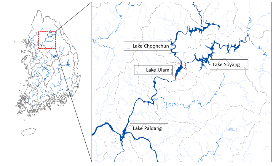
연구 대상지역은 최근 연이은 녹조 발생으로 수질관리 측면에서 주요 관심지역으로 부상되고 있는 북한강 수계 의암호로 수표면적 17 km2, 평균 너비와 길이는 각각 5 km, 8 km의 다목적댐이다. 유역면적은 7,709 km2이고 총 저수용량은 80,000,000 m3 이다.
2.2.1. 수질 분석
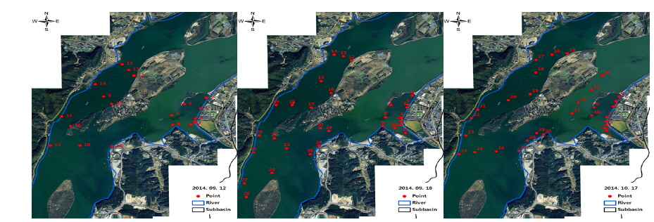
Chl-a 농도 추정모형 적용을 위해 1차(18개 지점, 2014. 9.12), 2차(30개 지점, 2014. 9.18), 3차(30개 지점, 2014. 10.17)에 걸쳐 현장 채수 및 Chl-a 농도를 분석하였다. 현 장채수는 춘천댐 방류수 유입구간과 공지천이 합류되는 소양댐 방류수 유입구간 및 합류구간을 중심으로 수행되었다 (그림 2). 샘플링은 보트를 이용해 표층수를 채수하였으며, GPS (Global Positioning System) 장비를 이용해 각 채수지점에 대한 위치정보를 취득하였다.
멸균채수병을 이용해 채수된 시료는 분석을 위해 빛이 들어오지 않는 아이스박스에 담아 실험실로 운송했고, 0.45μm GF/C 필터(Whatman)에 여과한 후 여지를 90% 아세톤과 10% 에탄올을 혼합한 용액을 이용해 색소를 추출하였다. 색소가 추출된 시료는 분광광도계(Spectrophotometer)를 이용해 흡광도를 측정한 후 수질오염공정시험법에 따라 측정된 흡광도를 Chl-a 농도로 환산하였다.
2.2.2. 현장 반사율 측정
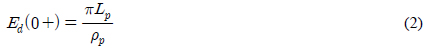
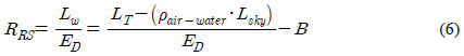
현장 채수와 병행하여 현장 분광복사계(Fieldspec4, ASD inc., USA)를 이용해 수체에서 복사되는 복사량(Ladiance, L (λ))과 복사조도(Irradiance, E(λ)), 반사율(Reflectance, R(λ))을 각각 측정하였다. 9월과 10월 측정시점의 평균 풍속은 0.9 m/s ~ 1.2 m/s로 비슷한 분포를 보였고, 반사율을 측정하는 동안 잔잔한 수면을 유지하였다. 다만 2차, 3차 측정시 운량은 각각 1.9, 0.8로 매우 맑았던 반면 1차 측정시 운량은 6.8로 상대적으로 구름이 많은 조건에서 반사율이 측정되었다. 물과 대기의 복사량(Lw, Lsky) 측정은 3° FOV(Field of view)를 갖는 fore optic 렌즈를 피스톨 그립에 장착해 측정했으며, 복사조도와 기준반사율 측정을 위해 cosine receptor와 99% 반사율을 갖는 원형 황산바륨판을 각각 사용하였다. 반사율 측정은 350 nm에서 2,500 nm 파장대를 1 nm 간격으로 측정하였고, 측정 당시 바람에 의한 노이즈 발생을 최소화하기 위해 지점별로 10회 측정된 값의 평균값을 사용하였다. 현장측정된 복사량 및 반사율 값을 이용해 원격반사도를 다음의 식으로부터 계산하였다.
Lw는 순수하게 물에 의해서 복사되는 복사량, Lt는 물에서 복사되는 전체 복사량, Lsky는 대기에서 입사되는 복사량이며, Ed(0+)는 아래 방향으로 입사되는 복사조도를 수표면 바로 위에서 측정한 값으로 다음의 식으로 표현 가능하다. ρp는 반사판을 이용해 측정한 기준 반사율이다.

2.2.3. 반사광 보정
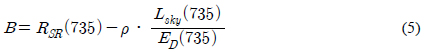
수표면에서 반사율 측정시에는 현장의 바람, 운량, 측정 각도등에 의해 반사광의 영향을 받게 된다. 측정된 결과값으로부터 순수하게 물에서 복사되는 반사율을 계산하기 위해 Zibordi et al. (2011)이 제안한 방법을 적용해 반사광 효과를 최소화하였다. 제안된 내용에 따르면 아래 식에서와 같이 표면반사율(Surface reflectance, Rsr)은 파장에 따라 값이 변하는 대기복사항(Sky radiance,

본 연구에서는 735 nm와 715 nm 파장에서의 현장 측정값을 이용해 표면반사율을 식 (4)로부터 산정하였다. 735 nm 파장에서 계산된 표면반사율을 이용해 식 (5)로부터 반사광에 의한 오차를 계산하고 식 (6)을 이용해 원격반사율을 산정하였다.

2.2.4. Red-NIR 3-band 모형 및 최적 파장 결정
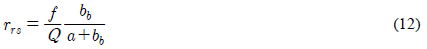
보통 물에서의 원격반사도는 아래 식 (7)로 표현 가능하다 (Gordon et al., 1988). 식 (7)에서 bb는 후방산란계수, a는 흡수계수, f는 입사광의 각도에 관련된 상수이며, Q는 BRDF (Bidirectional Reflectance Distribution Function) 계수이다.
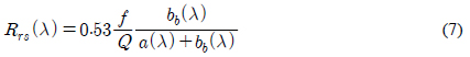
일반적으로 Chl-a 추정을 위한 3-band 모형은 적색 및 근적외 파장대의 좁은 파장대 정보를 이용하기 때문에 파장이동에 따른 f와 Q의 영향을 무시하는 경우가 많다. 또한 총 흡수계수는 조류와 순수한 물, CDOM, NAP에 의한 흡수의 합이라고 가정하였다. 아래 식에서 achla는 조류에 의한 흡수, aCDOM은 유색용존물질에 의한 흡수, aNAP는 조류 이외의 입자성물질에 의한 흡수, aw는 순수한 물에 의한 흡수를 의미한다.

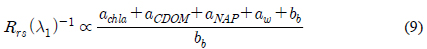
결국 식 (7)로부터 Chl-a 추정을 위한 첫 번째 파장에서의 반사율은 아래 식 (9)로 표현할 수 있다. 660 nm ~ 690 nm 파장 구간에서 선택된 첫 번째 파장은 Chl-a에 의한 흡수 피크가 나타나는 파장대이지만 Chl-a 이외에도 CDOM, NAP, 물에 의한 흡수와 후방산란에 영향을 받는 파장대이다.
두 번째 파장은 710 nm에서 730 nm 파장대에서 선택된다. 이 파장대에서 Chl-a에 의한 흡수는 첫 번째 파장에 비해 무시할 수 있을 만큼 작고, CDOM 및 NAP에 의한 흡수 또한 매우 작고 변화가 적다. 따라서 식 (8)과 식 (9)를 이용해 두 파장대에서 수체 내 물질들의 흡수와 산란 특성을 정리해보면 다음 식 (10)과 같다.
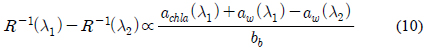
식 (10)에서 두 번째 파장의 선택으로 CDOM 및 NAP에 의한 영향은 최소화 했지만 여전히 후방산란에 의해 영향을 받고 있음을 알 수 있다. 따라서 후방산란의 영향을 최소화하기 위해 CDOM 및 NAP에 의한 흡수 효과가 미미하고 대부분의 흡수가 물에 의해서 결정되어 지는 740 nm에서 760 nm 파장구간에서 세 번째 파장을 선택한다.
본 연구에서는 이러한 과정을 거쳐 선택된 3-band 모형들 중에 MERIS (MEdium Resolution Imaging Spectrometer) 영상에 적용되었던 파장(665 nm, 708 nm, 753 nm)과 Gitelson등이 적용했던 파장(675 nm, 695 nm, 730 nm)을 이용해 의암호 Chl-a 농도를 추정하고 모형별 결과를 비교하였다.
또한, Gilerson et al. (2010)에 따르면 3-band 모형은 CDOM 및 NAP의 영향을 최소화하기 위해 근적외 파장대를 이용했기 때문에 두 물질의 농도 변화가 모형에 미치는 영향은 작지만 조류의 단위 투과거리당 흡수계수(specific absorption coefficient)와 Chl-a의 형광에 따른 양자수율 (quantum yield)이 변화함에 따라 모형의 정확도도 달라진다고 알려져 있다. 모형을 적용할 수체의 광학적 특성이 변하는 경우에는 사용되는 파장의 위치를 조정해 양자수율과 비흡수계수에 의한 영향을 최소화 할 수 있다(Dall’Olmo and Gitelson, 2006). 본 연구에서는 Chl-a 추정을 위한 최적 파장대 선정을 위해 각 모형에서 사용되었던 파장 위치를 초기값으로 입력하여 모형에서 추정된 Chl-a 농도와 실측한 농도를 비교해 각각의 파장대 구간에서 RMSE (Root Mean Square Error)를 계산함으로써 최적 파장대를 결정하였다.
2.2.5. 고유광특성 기반 Chl-a 추정
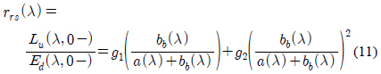
복사량과 반사율과 같은 외재적 광특성(Apparent Optical Properties, AOPs)은 수체 내에서 빛의 흡수와 산란과 같은 내재적 광학특성 또는 고유광학특성(Inherent Optical Properties, IOPs)으로 이루어진 함수로 표현 가능하다. 내재적 광특성들은 수체 내에서 빛의 전달과정을 결정짓는 가장 중요한 인자들이기 때문에 수체 내 구성물질의 정량적 분석을 위해 반드시 필요한 인자들이다(Hirawake et al., 2011; Le et al., 2009; Lee et al., 1996; Oliver et al., 2004; Wang et al., 2005). 최근 들어 현장에서 실측된 복사량, 반사율로부터 IOPs를 추정하기 위한 많은 연구들이 진행되었다(Garver and Siegel, 1997; Hoge and Lyon, 1996, 2005; Lee et al., 1996; Wang et al., 2005). 일반적으로 원격반사율로부터 IOPs를 추정하기 위한 알고리즘들은 원격반사율을 흡수와 산란의 함수로 표현한 아래 식 (11)에 기초를 두고 있다.

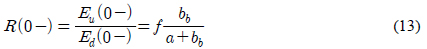
많은 연구들에서 식 (11)의 이차항을 생략함으로써 원격 반사율과 흡수, 산란의 관계를 식 (12) 또는 식 (13)으로 단순화시켜 사용해왔다(Brando and Dekker, 2003; Giardino et al., 2007; Hakvoort et al., 2002; Hoogenboom et al., 1998; Jupp et al., 1994; Kutser, 2004; Kutser et al., 2009; Zhang et al., 2009).

또한, GSM (Garver-Siegel-Maritorena) 모형(Garver and Siegel, 1997; Maritorena and Siegel, 2005, 2006; Maritorena et al., 2002), HL 모형(Hoge and Lyon, 1996, 1999, 2005), QAA (Quasi-Analytical Algorithm) 모형(Lee and Carder, 2004; Lee et al., 2002; Lee et al., 2009) 등과 같이 IOPs를 추정하기 위한 반경험적 또는 준분석 모형 알고리즘들이 개발되었다. 본 연구에서는 IIMIW (IOPs Inversion Model for Inland Waters) 모형(Li et al., 2013)을 이용해 IOPs를 산정하고(표 1), IOPs를 기반으로 하는 Chl-a 추정모형을 통해 의암호 Chl-a 농도를 추정하고 3-band 모형의 결과값과 비교하였다.
[Table 1.] Steps of IIMIW for deriving the inherent optical properties and Chl-a concentration
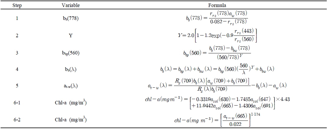
Steps of IIMIW for deriving the inherent optical properties and Chl-a concentration
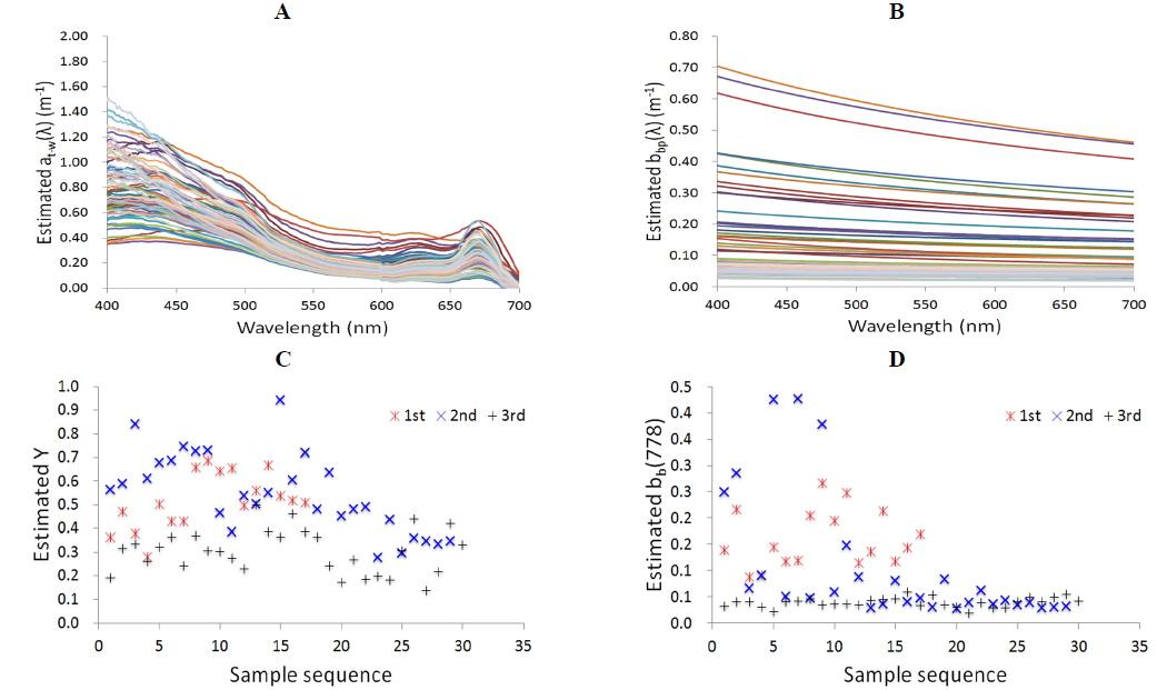
Chl-a이나 CDOM, NAP에 의한 흡수가 매우 작고 대부분 물에 의해 흡수가 일어나는 700nm 이후 파장대를 이용해 후방산란계수를 산정하였다(Gons, 1999; Gons et al., 2002; Gons et al., 2005; Gould et al., 2001; Le et al., 2009; Simis et al., 2005; Simis et al., 2007). 전체 파장대에 대한 후방산란계수와 입자성물질에 의한 산란계수는 표 1의 3~4 단계를 통해 산정 가능하다(Lee and Carder, 2004; Lee et al., 2002; Lee et al., 2009). bbw(λ)는 순수한 물에 의한 후방산란계수이고, Y는 입자성물질에 의한 후방산란계수를 산정하 기 위한 상수로 443 nm와 560 nm 파장에서 반사율 비로 계산된다(Lee et al., 2009). 물 이외의 물질들에 의한 흡수계수인 at-w(λ)는 709 nm 파장을 이용해(Gons et al., 2008; Gons et al., 2005; Simis et al., 2005; Simis et al., 2007) 산정한다. 순수한 물에 의한 흡수계수인 aw(λ)는 20°C 수온에서 실측된 값을 사용하였다(Buiteveld et al., 1994).
최종적으로 Ritchie (2008)가 제안한 식 (표 1, 6-1)과 Gilerson et al. (2010)이 제안한 식 (표 1, 6-2)으로부터 의 암호의 Chl-a 농도를 추정하고, 그 결과를 3-band 모형과 비교하였다.
모형을 통해 추정한 Chl-a 농도와 실측한 Chl-a 농도의 상대오차 비교를 통해 각 모형의 정확도를 평가했다. 또한 모형의 계통오차(systematic error)와 우연오차(random error) 평가를 위해 MNB (mean normalized bias)와 NRMS (normalized root mean square error)를 사용했다. 각각의 계산 방법은 아래 식과 같다.
[Table 2.] Statistics of chlorophyll-a concentration
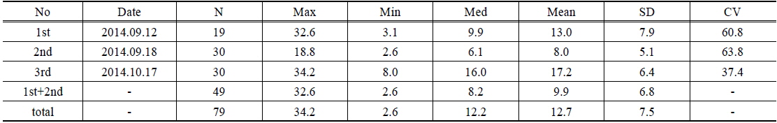
Statistics of chlorophyll-a concentration


3.1.1. Chl-a 농도 분포
Red-NIR 3-band 모형과 IOPs 기반 Chl-a 추정 모형의 결과와 비교·검증을 위해 3회(9.12, 9.18, 10.17)에 걸쳐 수질분석을 실시하였다. 전체 자료에서 Chl-a 농도는 최소 2.6 mg/m3에서 최대 34.2 mg/m3의 분포를 나타냈고, 1, 3차 측정 결과에 비해 2차 측정 결과가 상대적으로 낮은 분포를 보였다.
3.1.2. 원격반사율 및 반사광 보정
의암호 수표면 위에서 측정된 1차(A, D), 2차(B, E), 3차(C, F) 총복사량(total radiance, LT)에 대해 반사광 보정계수 (
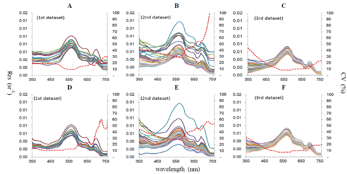
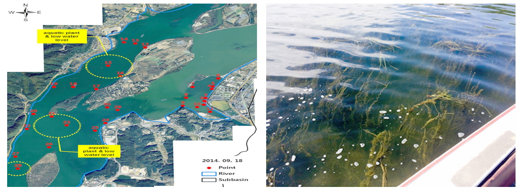
전체적으로 측정된 반사율 패턴은 400 nm와 650 nm ~ 700 nm 파장대에서 Chl-a에 의한 높은 흡수로 낮은 반사율을 보이고, 반사율 피크의 위치 등은 유사한 경향을 보이지만 1, 3차에 측정된 반사율에 비해 2차에 측정된 반사율이 전 파장대에 걸쳐 큰 변화를 보이고 있음을 확인할 수 있다. 또한, 청색파장대(400 nm ~ 500 nm)에서보다 녹색파장대 (500 nm ~ 600 nm)에서 높은 반사율을 보이고 있으며, 2차측정의 경우에는 측정지점에 따라 550 nm 파장에서 반사율이 0.002 ~ 0.014 sr-1로 약 7배 차이를 보였다 (B, E).
일반적으로 녹색 및 청색파장대의 반사율은 Chl-a 뿐 아니라 CDOM에 의한 흡수와 NAP에 의한 흡수, 산란의 영향을 받고 있어 녹색 및 청색 파장을 이용한 Chl-a 추정 모형은 탁도가 높은 담수역에는 적합하지 않은 것으로 알려져 있다. 또한 적색 파장대(600 nm ~ 700 nm)에서는 남조류에 의한 흡수로 625 nm에서 낮은 반사율과 Chl-a에 의한 흡수로 675 nm 파장에서 낮은 반사율을 보이지만 (Sims et al., 2005), 조류에 의한 흡수와 함께 다른 물질들에 의한 흡수와 산란의 영향을 동시에 받는 파장대이다. 하지만 의암호에서 측정된 반사율 스펙트럼에서는 625 nm 파장에서 반사율 피크가 관찰되지 않는 반면 675 nm 파장대에서 낮은 반사율과 690 nm에서 710 nm 사이에 높은 반사율을 보이고 있어, 측정 당시 남조류에 의한 영향은 적었던 것으로 추정된다. 아울러 690 nm에서 710 nm 파장대에서 눈에 띄는 반사율 피크는 Chl-a 농도가 5 mg/m3 이상인 수체에서 공통적으로 관찰되는 현상이며, Chl-a 농도가 높을수록 피크 파장대는 710 nm에 가까워지는 특징을 보인다.
3.2.1. Red-NIR 모형을 이용한 Chl-a 농도 추정
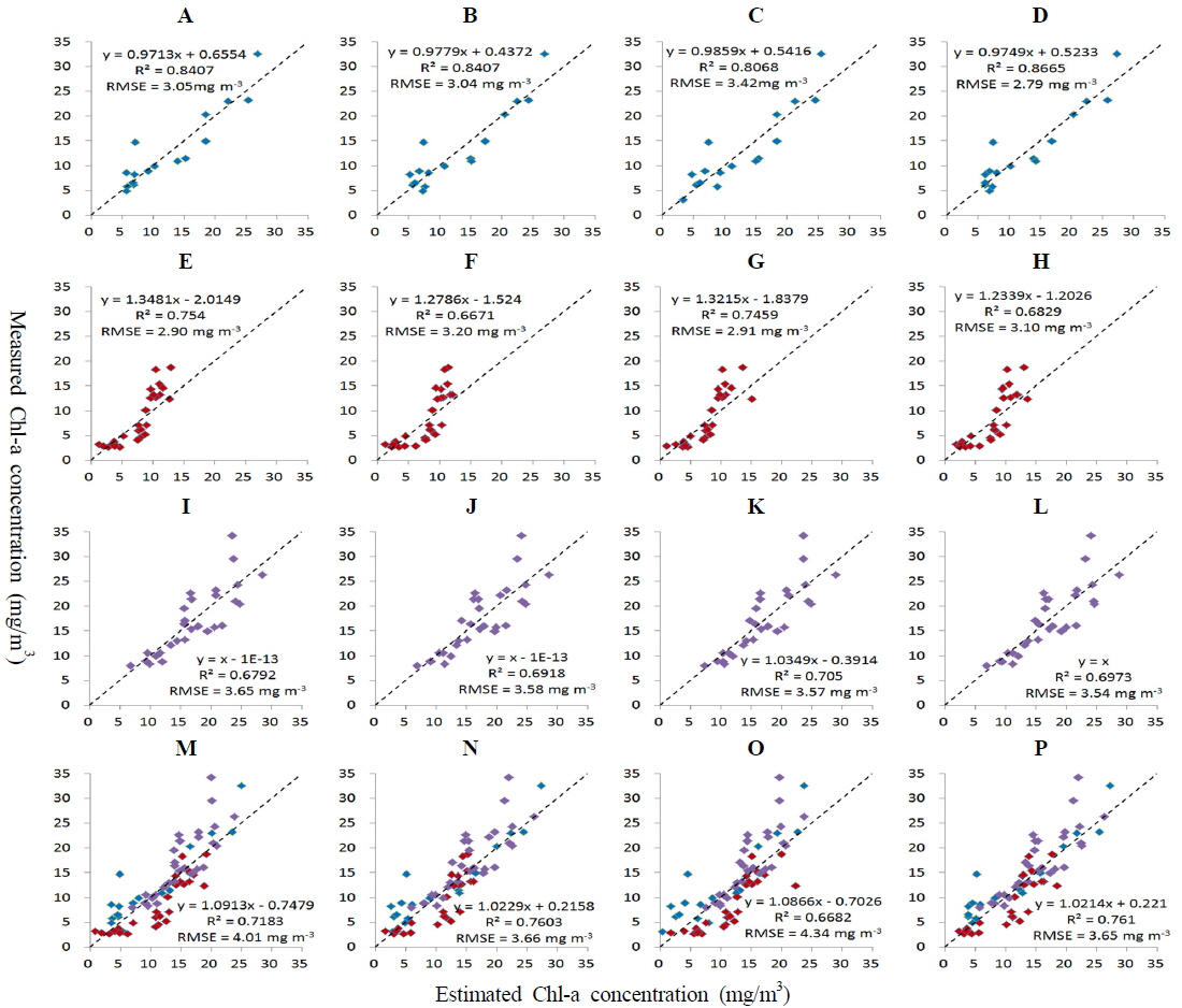
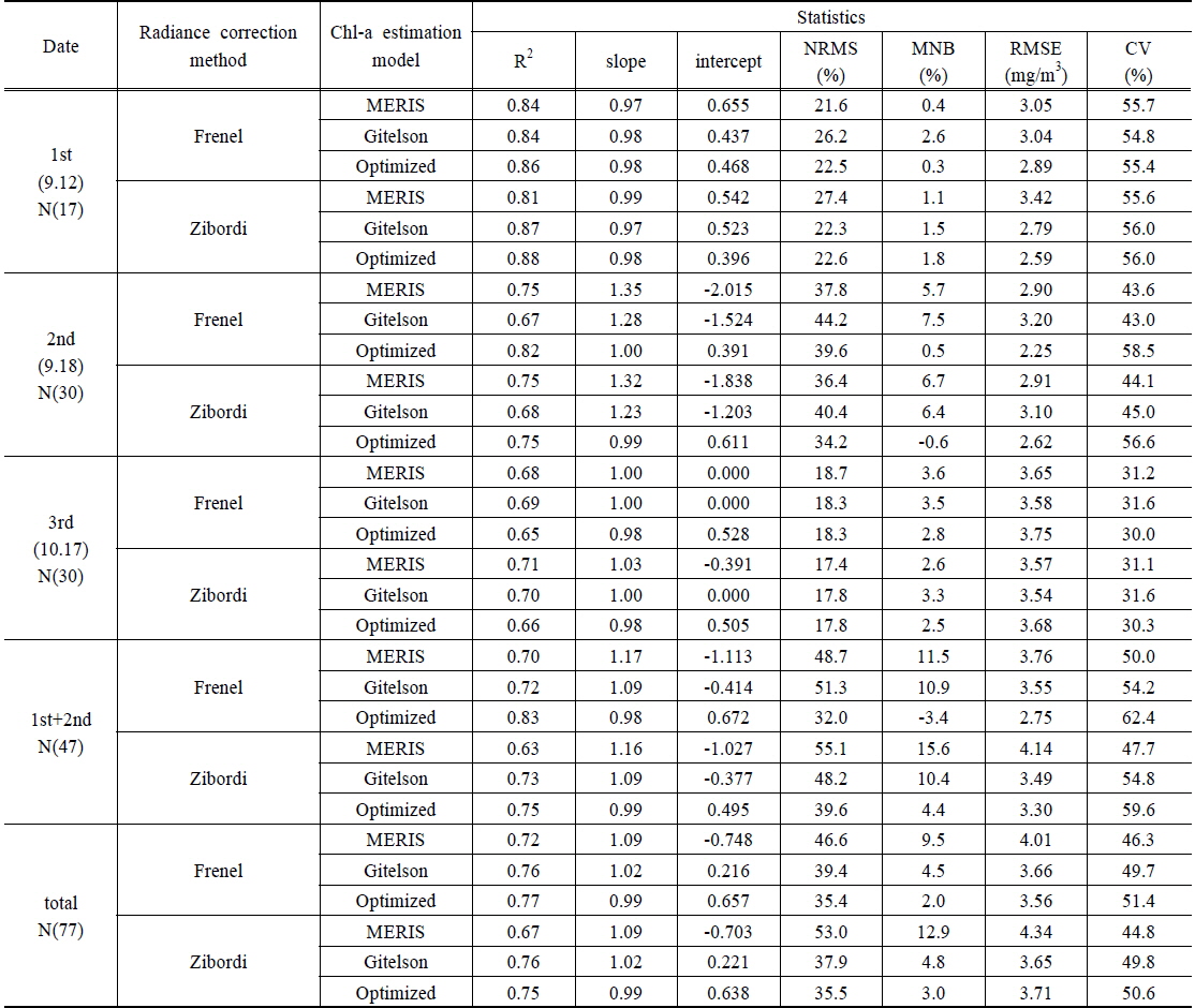
1차 측정 (2014.9.12.)한 반사율 자료에 Red-NIR 3-band 모형을 적용한 결과, 복사량을 보정한 원격반사율에 MERIS 영상에 적용되었던 3-band(665 nm, 708 nm, 753 nm)를 이용한 방법(D)의 RMSE가 2.79 mg/m3으로 가장 낮았고, 전반적으로 결정계수가 0.84에서 0.87로 실측된 Chl-a 농도를 잘 재현하였다. 보통 Chl-a 농도가 낮은 경우에는 상대적으로 CDOM과 NAP에 의한 흡수 영향이 커져서 모형의 정확도가 낮아지는 것으로 알려져 있지만 의암호 1차 측정자료는 낮은 Chl-a 농도에서도 모형의 예측치와 실측치가 유사한 결과를 보이고 있어 측정 당시 CDOM과 NAP의 영향이 적었던 것으로 판단된다. 2차 측정자료(2014.9.18.)에 3-band 모형을 적용한 결과, 반사광 보정계수를 이용해 산정된 원격반사율에 MERIS 영상에 적용되었던 3-band를 적용한 방법(E)의 RMSE가 2.90 mg/m3으로 가장 낮았고 결정계수는 0.68에서 0.75의 분포를 보였다. 2차 측정자료 중에서 모형을 적용해 산정된 결과값과 실측한 Chl-a 값을 비교하여 상대오차(є
3차 측정자료(2014.10.17.)는 Zibordi et al. (2011)이 제안한 방법을 이용해 복사량을 보정한 원격반사율에 MERIS 3-band를 적용한 방법(L)의 RMSE가 3.54 mg/m3으로 가장 낮았고, 전반적으로 결정계수가 0.68에서 0.71의 범위를 보였다. I, J, K, L의 우연오차에 의한 불확도는 각각 18.7%, 18.3%, 17.4%, 17.8%로 나타났고, 계통오차에 의한 불확도는 각각 3.6%, 3.5%, 2.6%, 3.3%로 나타났다. 일반적으로 Chl-a의 농도가 10 mg/m3 이하인 경우에는 Chl-a 추정 모형의 오차에 의한 불확도가 증가하는 것으로 알려져 있지만 3차 측정된 Chl-a의 최소 농도가 8 mg/m3으로 1, 2차 측정자료에 비해 상대적으로 높아 오차에 의한 불확도가 낮게 나타났다.
전체 측정자료(1차, 2차, 3차)에 3-band 모형을 적용한 결과, 복사량 보정과정을 거친 원격반사율에 Gitelson 등이 사용했던 3-band(675 nm, 695 nm, 730 nm)를 적용한 방법(P)의 RMSE가 3.65 mg/m3으로 가장 낮았고, 결정계수는 0.67에서 0.76의 범위를 보였다.
3.2.2. 최적파장대 선정 및 Chl-a 농도 추정
최근까지 700 nm 파장대에서 나타나는 반사율 피크를 이용해 혼탁수체에서 Chl-a 농도를 추정하기 위한 많은 연구들이 수행되었다(Gitelson et al., 1985; Gower et al., 1999; Stumpf and Tyler, 1988; Vasilkov and Kopelevich, 1982). 대부분의 연구들에서 Chl-a 농도 추정을 위해 670 nm 파장에서의 반사 피크나 R705/R670 (Dekker, 1993; Gitelson et al., 1985; Gitelson and Kondratyev, 1991; Han and Rundquist, 1997; Mittenzwey et al., 1992)과 같은 반사율비 또는 피크가 나타나는 파장의 위치정보(Gitelson, 1992)를 이용하고 있다. 최근에는 육생식물에 포함된 색소량 추정을 위해 개발된 3-band 모형(Gitelson et al., 2003; Gitelson et al., 2005)이 혼탁수체에서 Chl-a 농도를 추정하는데도 적합하다는 연구결과가 Dall’Olmo et al. (2003)에 의해 제시되었다. 또한, 3-band 모형에 영향을 주는 많은 인자들 중에서 조류의 비흡수계수(specific absorption coefficient)와 Chl-a의 형광에 따른 양자수율(quantum yield)이 모형의 정확도에 미치는 영향이 상대적으로 크다는 사실이 밝혀졌다 (Dall’Olmo and Gitelson, 2006). 결국 수체의 광학적 특성이 변하는 경우에는 모형에서 사용되는 파장의 위치를 조정해 양자수율과 비흡수계수에 의한 영향을 최소화하는 과정이 필요하다는 사실을 시사하고 있다.
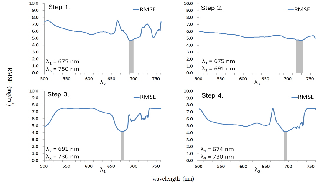
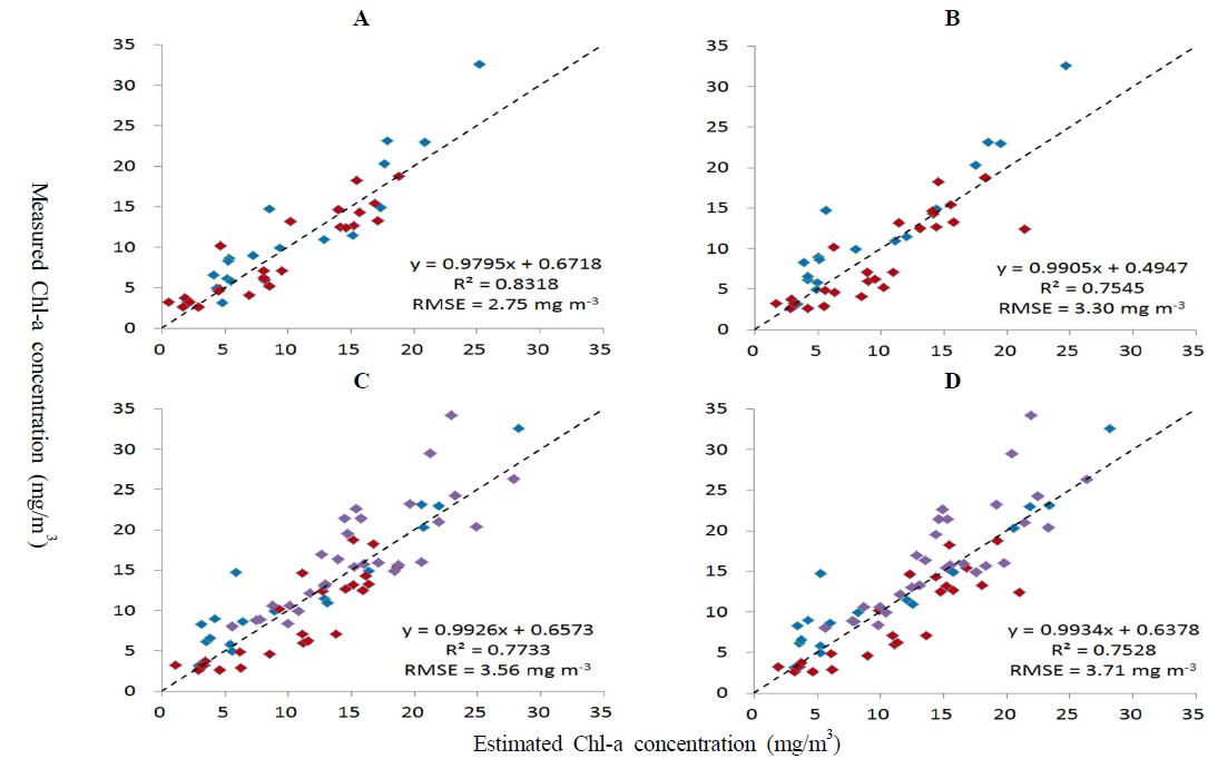
따라서 본 연구에서는 1차와 2차에 측정된 자료와 전체 자료에 대해 최적 파장을 선정하였다. 최적 파장 선정을 위해 초기 파장을 임의로 입력한 3-band 모형을 이용해 추정한 Chl-a 농도와 실측한 결과값을 비교하여 400 nm에서 800 nm 파장대 구간에서 반복계산을 통해 1 nm 간격으로 RMSE를 계산한 후 RMSE가 최소가 되는 파장구간의 평균값을 최적파장으로 선정하였다(그림 6).
최적화 과정을 거쳐 선정된 파장들을 이용해 현장에서 측정된 자료에 대해 Chl-a 농도를 추정하였다(그림 7). MERIS 3-band & glint correction coefficient(A), MERIS 3-band & Zibordi correction(B)를 적용한 1, 2차 측정자료의 보정 전과 후의 RMSE는 각각 3.76 mg/m3에서 2.75 mg/m3, 4.14mg/m3에서 3.30 mg/m3으로 감소되었다. 또한, MERIS 3-band & glint correction coefficient(C), MERIS 3-band & Zibordi correction(D)를 적용한 전체 측정자료의 보정 전과 후의 RMSE는 각각 4.01 mg/m3에서 3.56 mg/m3, 4.34 mg/m3에서 3.71mg/m3으로 감소되는 결과를 보였다.
Dall’Olmo and Gitelson (2006)은 수체의 광학적 특성이 변할 때 최적파장 선정을 통해 Chl-a 농도 추정을 위한 3-band 모형에 미치는 영향을 최소화할 수 있다고 했지만, 본 연구결과에서는 9월 중순에서 10월 중순 사이에 측정한 의암호 Chl-a의 농도 분포가 유사했고 각 측정 시기에 수체의 분광학적 특성변화가 적었기 때문에 보정 전·후 모형의 정확도 변화가 선행연구 결과들과 비교했을 때, 상대적으로 큰 차이를 보이지 않았던 것으로 판단된다.
현장 실측된 Chl-a 농도와 본 연구에서 적용한 3-band 모형 및 최적파장을 이용해 산정된 Chl-a 농도에 대한 비교결과를 표 3에 제시하였다. 전체 측정자료에 대해 예측된 Chl-a 농도는 2.6 mg/m3에서 34.2 mg/m3까지 변화를 보이고, 예측치의 RMSE는 2.1 mg/m3에서 4.34 mg/m3까지 변화하고 있으며, Chl-a 추정을 위한 예측모형의 우연오차에 의한 불확도는 17.4%에서 55.1%, 평균 오차는 0.3%에서 15.6%의 결과를 나타냈다. 또한, Chl-a 추정에 사용된 측정자료와 적용 모형의 30개 조합에서 모형 보정을 통해 최적파장을 선정한 방법이 상대적으로 높은 정확도를 보이는 것을 확인할 수 있었다.

Results of the 3-band algorithm validation with each dataset and the remote-sensing spectra. NRMS is the normalized root mean square error, MNB is the mean normalized bias and CV is the coefficient of variation. All parameters are statistically significant (p<0.0001).
최근 들어 AOPs를 이용해 IOPs를 산정하기 위한 연구들이 활발하게 추진되고 있지만(Garver and Siegel, 1997; Hoge and Lyon, 1996; Le et al., 2009; Lee et al., 1996; Wang et al., 2005), 대부분 연구들이 해양을 대상지역으로하고 있어 상대적으로 내륙 호소나 하천에 적용할 수 있는 변환모형에 대한 연구는 미흡한 실정이다. 따라서 본 연구에서는 다양한 수리학적 특성을 보이는 수체에 대해 여러시기에 보다 안정적으로 Chl-a 추정이 가능하도록 하기위해 IOPs Inversion Model of Inland Waters (IIMIW, Linhai Li et al., 2013)를 이용해 현장측정된 AOPs 정보들을 이용해 IOPs를 산정하였으며, 이를 기반으로 Chl-a 농도를 추정하고 그 결과를 3-band 모형의 결과와 비교하였다.
일반적으로 조류가 과성장하는 시기의 수체에서는 Chl-a에 의한 흡수로 443 nm와 675 nm 파장에서 큰 흡수 피크를 보이지만 계산된 at-w(λ) 스펙트럼들은 400 nm 파장대에서 뚜렷한 흡수 피크가 관찰되지 않고 적층된 형태를 띄고 있어 Chl-a와 CDOM에 의한 흡수 영향을 동시에 받고 있는 것으로 판단된다. 또한, 뚜렷한 흡수피크가 보이지 않고 지수감소하는 형태를 보이는 스펙트럼들은 CDOM에 의해 흡수가 지배적이었기 때문이다.
Kutser et al. (2009)과 Ma et al. (2009), Sun et al. (2010)의 연구결과에 따르면 다양한 시기에 측정된 후방산란계수는 0.05 m-1 ~ 10 m-1 범위로 수 백배에서 수 천배 차이를 보이는 것으로 알려져 있다. 하지만 의암호에서 산정된 총 산란계수(B)는 0.02 m-1에서 0.7 m-1까지 약 30배 정도의 차이를 보이고 있으며, 이는 의암호 AOPs 측정시기가 9월 중순에서 10월 중순까지 약 1개월 동안 비교적 짧은 시기에 이루어졌고, 각 측정시기에 수체의 물질구성과 광학적 특성들이 유사했기 때문으로 해석된다.
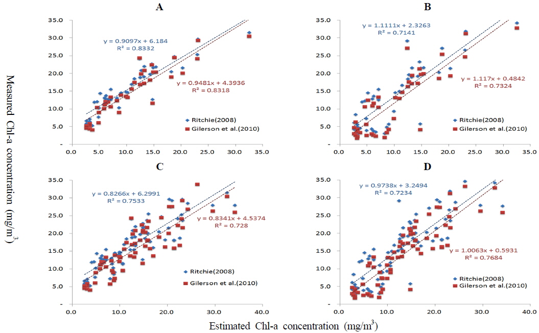
변환 모형을 통해 산정된 IOPs를 이용해 Ritchie (2008)가 제안한 방법과 Gilerson et al. (2010)이 제안한 방법을 적용해 산정된 Chl-a 농도와 실측값을 비교하였다 (그림9). 적용된 두 식 모두 3-band 모형에서 CDOM 및 NAP에 의한 흡수 영향을 최소화하기 위해 사용되었던 근적외 파장대를 사용하지 않았음에도 3-band 모형 적용 결과와 비슷하거나 나은 정확도를 보이고 있어 계산된 IOPs 값이 유효했음을 확인할 수 있었다.
하지만 앞서도 언급한 것처럼 3-band 모형 및 IOPs 기반 예측모형에 사용된 Chl-a 측정자료가 9월 중순에서 10월 중순 사이의 제한된 시기에 측정되었기 때문에 두 모형 간 예측 정확도가 비슷한 결과를 보였지만, 보다 다양한 시기에 관측된 자료를 추가할 경우 IOPs 기반 모형이 상대적으로 높은 정확도를 보일 것으로 판단된다.
본 연구는 초분광센서를 이용해 넓은 수체에서 동시다발적으로 발생되는 녹조현상을 원격으로 모니터링 하기 위한 방법론을 정립하기 위해 진행되었다. 이를 위해 최근에 Chl-a 추정을 위해 개발된 Red-NIR 3-band 모형들을 이용해 의암호 Chl-a 농도를 추정하고 현장 실측자료와 비교함으로써 적용성을 검토하였다. 또한, 3-band에서 사용되는 파장대를 최적화하여 시기 변화에 따른 모형의 정확도 변화를 최소화하고자 하였다. 끝으로 현장에서 실측된 반사율, 복사량과 같은 AOPs를 이용해 수체 내에서 발생되는 흡수와 산란 등과 같은 IOPs 정보들을 유추하고 IOPs를 기반으로 하는 Chl-a 추정모형을 적용하여 3-band 모형 결과와 비교하였다.
MERIS 영상에 적용되었던 3-band (665 nm, 708 nm, 753 nm) 모형과 Gitelson이 제안한 3-band (675 nm, 695 nm, 730 nm) 모형, 최적 파장대를 선정한 3-band 모형 등 전체 30개 방법을 이용해 의암호 Chl-a 농도를 추정한 결과, 결정계수는 0.65에서 0.88까지 변화를 보였고 RMSE는 2.25 mg/m3에서 4.34 mg/m3까지 값을 보여 전반적으로 실측된 Chl-a 농도와 비슷한 추정결과를 보였다. 또한, 1차, 2차, 3차 및 전체 측정자료에 적용된 각각의 Chl-a 추정 방법에서 최적화 과정을 거쳐 선정된 3-band를 이용한 방법이 상대적으로 RMSE가 작게 나타났다. 일반적으로 Chl-a 농도가 낮은 시기에 밴드조합을 통한 Chl-a 추정모형은 정확도가 떨어지는 것으로 알려져 있지만(Gons et al., 2008), 최적파장대를 이용한 3-band 모형은 Chl-a 농도가 5 mg/m3 이하인 경우에도 실측 수질과 유사한 결과를 보이고 있어 동일 수체에 대해 연중 조류의 공간적 분포 모니터링이 가능할 것으로 판단된다. 하지만 본 연구에서 측정된 조류의 농도는 35 mg/m3 이하로 비교적 낮은 수준을 보이고 있어 향후 보다 다양한 시기에 측정된 자료를 추가하여 높은 농도 조건에서 조류의 광학적 특성과 농도간의 상관관계 또한 규명할 필요가 있을 것으로 판단된다.
끝으로 현장에서 측정된 AOPs를 이용해 IOPs를 계산한 결과, 비슷한 시기의 짧은 기간 동안에 측정된 자료로 인해 큰 변화를 보이지 않았으며, 계산된 at-w(λ) 스펙트럼들에서 뚜렷한 흡수 피크가 관찰되지 않고 적층된 형태를 보여 Chl-a와 CDOM의 영향을 동시에 받고 있었던 것으로 확인됐다. 또한, IOPs를 이용한 Chl-a 추정결과는 3-band 모형을 이용한 결과와 비교할 때, 적용된 자료에 따라 RMSE가 평균 18%에서 33.6%까지 감소하였으며 다양한 시기에 측정된 자료를 추가해 분석할 경우 두 모형의 정확도 차이는 더 커질 것으로 예상된다. 또한 마이크로시스티스, 아나베나, 오실라토리아, 아파니조메논 등과 같이 여름철에 주로 출현하는 유해남조류의 효과적인 관리를 위해서는 남조류 세포수와 조류의 흡수특성, 피코시아닌 농도와 조류의 흡수특성 등에 대한 추가적인 연구가 필요할 것으로 판단된다.