Polarization is a coherent characteristic of the electromagnetic (EM) wave in a medium. In a plane wave, both the electric field vector and magnetic field vector of the electromagnetic radfield vectoriation always oscillates parallel to a fixed direction in space. Light of such character is said to be linearly polarized, and maintains a constant direction of oscillation, and does vary spatially in a regular manner, producing either elliptically polarized or circularly polarized light (Fowles 1975; Jackson 1975; Pedrotti & Pedrotti 1987). Polarization characteristic have been used in radio transmission to reduce interference between channels, particularly at VHF frequencies and beyond (Masayoshi 2007; Yao et al. 2007). Free-space communication has forced the use of circular polarization, which has the fundamental advantage of precluding disturbance from the reflections of signals (Leitch et al. 2002; Elser et al. 2009). Free-space optical (FSO) communication utilizes a spatial diversity receiver to receive the binary signals, which are modulated by two circular polarizations. FSO communication employing a binary polarization shift keying coherent modulation scheme are utilized in atmospheric turbulence channel (Tang et al. 2010) and free-space quantum key distribution (QKD) by rotation-invariant twisted photons are used to guarantee unconditional security in cryptographic communication (Vallone 2014). On 17 March 2014, astronomers from the Harvard Smithsonian Center for Astrophysics announced their detection of signature patterns of polarized light in the Cosmic Microwave Background (CMB) (Ade 2014; Calvin 2014; CfA 2014). The team hunted for a special type of polarization called ‘B-mode’ which represents a twisting or ‘curl’ pattern in the polarized orientations of the ancient light. This is the strongest confirmation yet of the cosmic inflation theory (Boyle 2006). Gravitational waves squeeze space as they travel, and the squeezing produces a distinct pattern in the CMB. Gravitational waves have a “handedness” much like light wave and can have left- and right-handed polarization.
In the Standard Model, the weak bosons (W±, Z) mediate the weak interactions between different flavors (all quarks and leptons). Experimental results have shown that all produced and observed neutrinos have left-handed helicity, and all antineutrinos have right-handed helicity (Aad et al. 2012; CfA 2014). The helicity of the elementary particle could be a keyword to determine the Standard Model.
The scope of application of polarization has expanded explosively this decade with the development of communication technology. Accordingly, it is fundamentally important for application of a manipulation scheme to understand the physics of polarization’s conception and the process of producing polarization modes. Presently the definition of polarization has been modified, and its nomenclature upgraded, which can be confusing to students of physics and researchers. For instance, there are similar customary nomenclature for the right circularly polarization: right circularly (Fowles 1975; Jackson 1975), right-circularly (Pedrotti & Pedrotti 1987), right-hand circularly (Reitz et al. 1993), and right-handed (Born & Wolf 1999; Georgi 1982) circularly polarization. Right circularly polarization and right-handed polarization are different types of polarization, although with similar names. Recently, the visualization of polarization propagating in matter has drawn physicist's attention for potential applications in modern physics and information technology (Tamm 1997; Mooleskamp & Stokes 2015; Yun & Choi 2013).
We have provided a dynamic polarization modes platform for simulating polarization modes with Jones matrices calculations, corresponding to the physical arrangement of optical elements, in a
2. MATHEMATICA SIMULATION FOR THE CONVERTING POLARIZATION MODES
2.1 Electromagnetic waves in solids
The propagating process of electromagnetic waves in solids is different from that in the vacuum, since and of the electromagnetic waves interact with the electrons in a solid (Pedrotti & Pedrotti 1987; Fowles 1975). In particular, although the electromagnetic waves are an harmonic plane wave, the fields may pull or push the electrons in the orbital of a solid, which is responsible for inducing dipole moment and magnetization im the solid. If we assume that the medium is not a magnetic material and , the Helmholtz wave equation in a solid (Fowles 1975; Jackson 1975) is

where . If we suppose the EM wave will be a form of solution such as , we can rewrite Eq. (1) using a wave vector

It then becomes a vector equation for , which indicates that the propagation process varies with the component of electric susceptibility

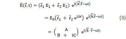
Aa shown above, field vector may be presented as the Jones vector (Jones 1941) with a complex vector amplitude {A, B ± iC} oscillating in an inhomogeneous plane. The wave vector and form a real mutually orthogonal unit vectors . Here is a complex wave vector and N = n + iκ is the complex refraction index. For Eq. (3) to be a solution of Eq. (2) as a homogeneous plane harmonic wave, it should be, . Then we get the relations: , and , which result in propagation speeds that are different along the direction in the medium. Therefore, there will be a cumulative phase difference Δ
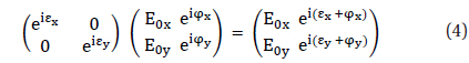
A quarter wave plate is a thin birefringent crystal the thickness of which has been adjusted to produce a ±

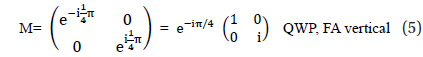
where εx and εy represent the advance in phase of Ex - and Ey - component of the incident light. As an example, consider a quarter-wave plate (QWP) which makes Δ

This is the case of fast axis vertical (FA vertical). Similarly, we can determine the corresponding Jones matrix for a half-wave plate (HWP) or eighth-wave plate (EWP) or arbitrary phase of retarded. Jones matrices derived for various wave plates are summarized in Table 1.
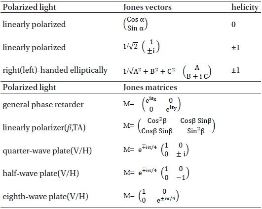
Summary of Jones vectors in the most common and Jones matrices of the wave plates and phase retarders (Pedrotti & Perotti 1987).
We desire now to create a new simulation presenting a means of producing polarizing modes from a Jones calculation corresponding to the physical arrangement of optical elements in the
2.2 Polarization modes Mathematica simulation
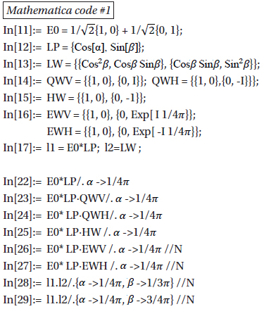
We have used


where, , , and ard both complex vectors and , and are real vectors with where is a magnetic intensity vector in the matter. We examine the process of generating polarzation modes with the normalized Jones vectors calculations in the
The
2.3 Helicity of the elliptically polarized wave
The handedness of an elementary particle depends on the correlation between its spin and its momentum (Goldhaver et al. 1958). If the spin and momentum are parallel, the particle can be said to be right-handed or have a helicity of 1. If they are anti parallel, the particle is left-handed or have a helicity of -1. We may also adopt this definition to modern optics, since the circularly polarized electromagnetic wave is just a helical motion with helicity. The helicity of the polarized electromagnetic wave is a critical factor in modern communication technology and photonics (Aad et al. 2012; Goldhaver et al. 1958; Rubenhok et al. 2013). However, determination of the helicity is a perplex issue because we need to aware of the vectorial behaviors accurately unless we may observe propagating polarized wave (Goldhaver et al. 1958). Therefore, it is very helpful to simulate advanced polarization modes in the medium, and further, it would be more helpful to evaluate the helicity operator in a physics state.
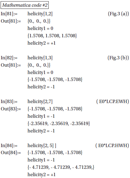
Here we simply estimate the helicity with a calculation of phase shift in the process in the

The helicity[1, 2] returns two helicities with two lists of three phase differences in the two divisions for the optical device arrangement of linearly polarizer (JvC=1) and quarter-wave plate (JmC=2). The helicity[2, 7] returns the helicities of the optical arrangement of left-circularly polarizer (JvC=2) and eighth-wave plate (JmC=7). It needs to be noticed that the three phase differences are all 1.5708 (
3. DYNAMIC POLARIZATION PLATFORM WITH JONES VECTORS IN MATHEMATICA
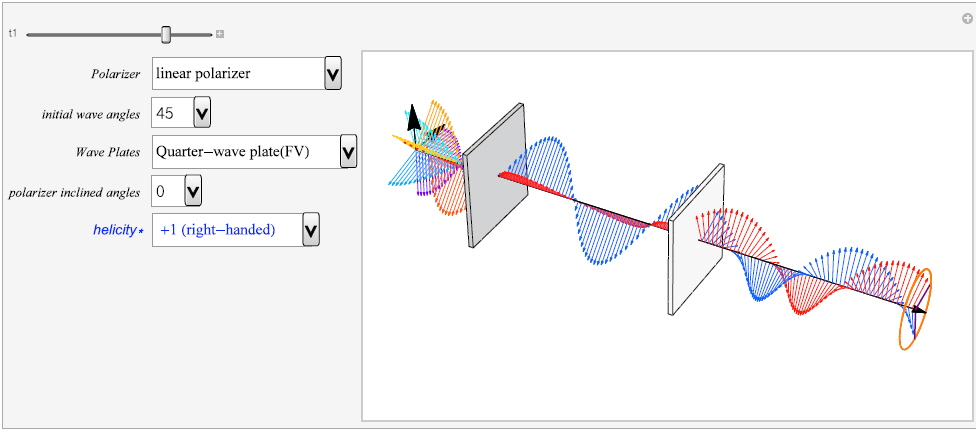
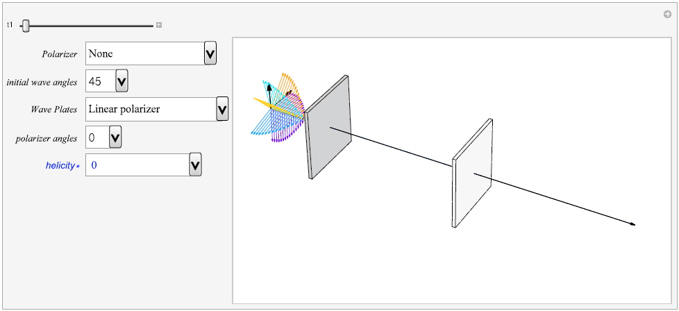
We have provided a dynamic polarization platform with Jones vectors (jdpmp) in the Graphics3D in
The platform starts by clicking the button ▶ on pop up ⊕ of the
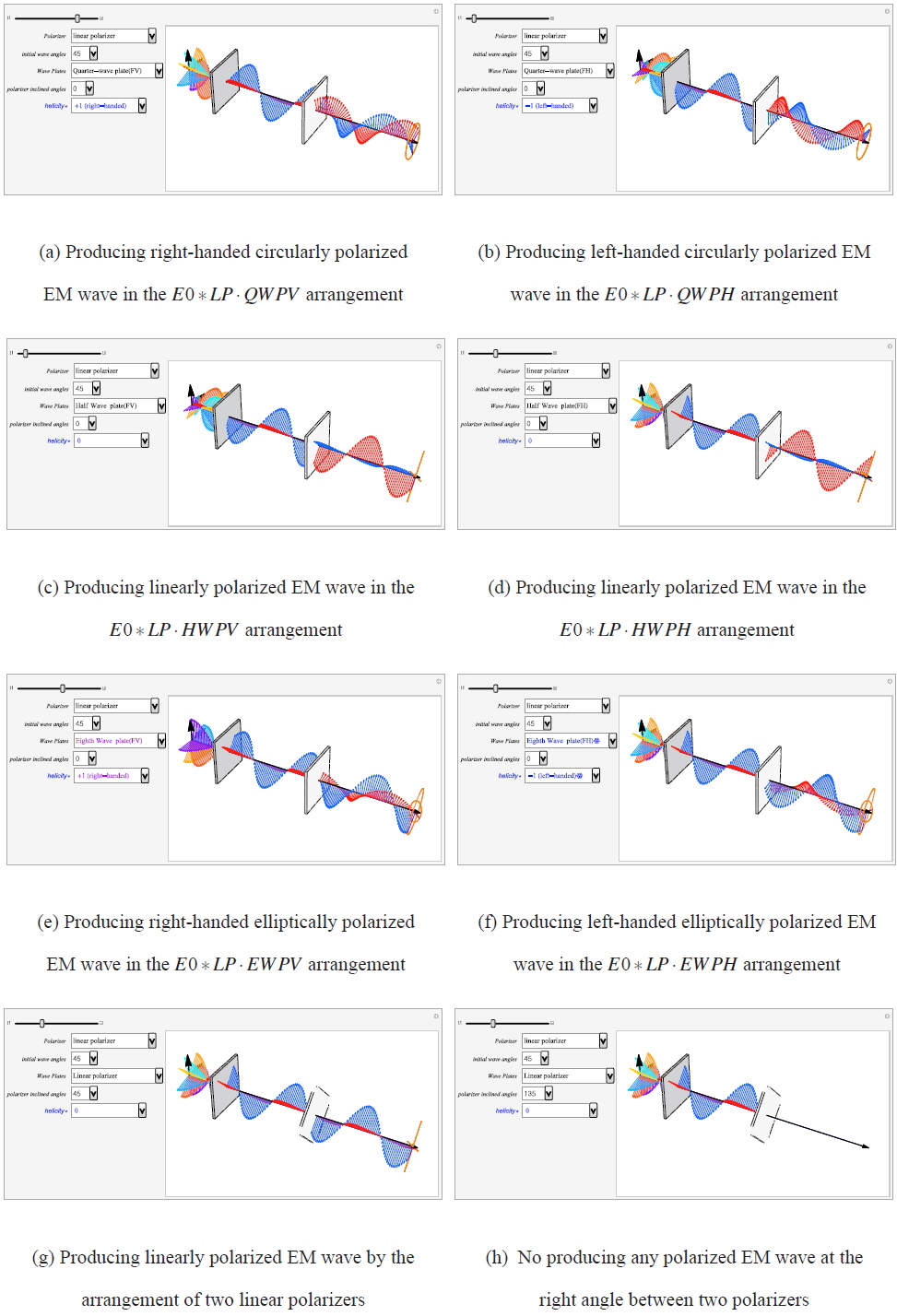
Fig. 3 shows snapshots of three kinds of polarization modes. Figs. 3a and 3b shows a circularly polarization mode, Figs. 3c and 3d linearly polarization, Figs. 3e and 3f elliptically polarization according to the arrangement of optical devices. If we utilize linear polarizer JmLinear [
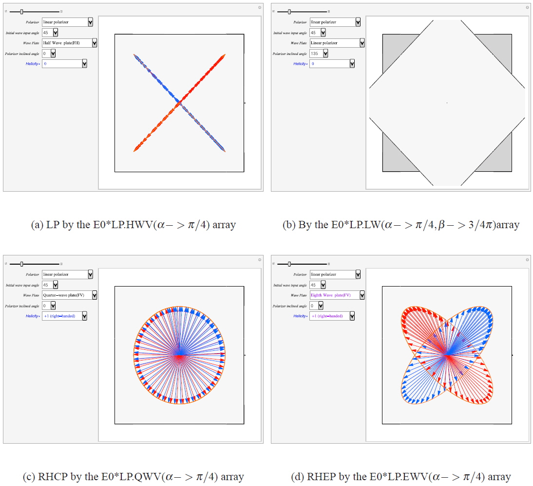
Fig. 4 presents snapshots of three kinds of polarization modes viewed in the ViewPoint (200, 0, 0) against the propagation direction for confirmation of the transverse behavior and progression of the Poynting vector. It shows the orthogonal transverse of the propagating process of the waves and confirms the flow of Poynting vector. This is the visualization of the graphic version of satisfying Maxwell’s vector equations Eqs. (6) and (7). The traces of both and are dynamically shown in the polarization modes at the edge of the
The platform will run faster or slower and stop and restart again by clicking the pop-up menu of the tl panel for more analytical observations while the polarization mode is running. During the platform stop, you will change to another mode only if you click a panel, then the changed mode will be presented automatically. At that time you can save the presenting mode or print out the mode status. While the platform is running, you can confirm the helicity by observing the spin direction of the field vectors along the orange trace of the helical propagation of the and vector fields at the edge of the platform. The helicities on the
As far as we know, other than
We have provided a dynamic polarization mode platform,