The Particle-In-Cell (PIC) method is a technique commonly used to simulate the dynamics of charged particles interacting with electromagnetic fields. Since the 1950s, the PIC method has been used for self-consistent kinetic simulations along with the Vlasov simulation method. The PIC method is useful to study the dynamics of plasmas that takes place on spatial and temporal scales that magnetohydrodynamics (MHD) cannot handle properly.

In this paper, we present the development of a 2.5-dimensional relativistic electromagnetic PIC code. The code is developed to study electromagnetic phenomena that occur in space plasmas. To test this newly developed code, we performed simulations for both electrostatic and electromagnetic phenomena and compared the results with those of two widely used codes (Umeda 2004, Gary et al. 2011). For the test of the electrostatic phenomena, we applied the code to electron two-stream instabilities. For the electromagnetic phenomena, whistler instabilities driven by electron temperature anisotropy were simulated.

In section 2, we briefly introduce the numerical schemes adopted in the code, and in section 3, we present test simulation results in comparison with those reported previously. Discussions and conclusions are presented in section 4.

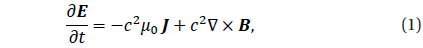
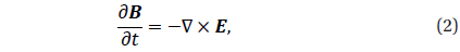
To handle various plasma processes we solve Maxwell’s equations and relativistic Lorentz force equation as follows:

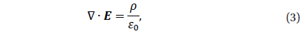
where E, B, J, and ρ are electric field, magnetic field, current density, and charge density, respectively. Lorentz equation, q_i, m_i, v_i, and γ_i are charge, rest mass, velocity, and Lorentz factor of the i-th particle, respectively. Maxwell’s equations describe the variation of electromagnetic fields, which the motion of charged particles through Lorentz force equation. Particles contribute to Maxwell’s equations by the charge and current densities.

When particles are initially loaded into the simulation domain using uniform random distribution, electric field can be produced by the non-uniformity in charge density caused by the random distribution. Thus, we first solve Poisson equation,

where φ is the electrostatic potential used to obtain the initial electric field. To solve the Poisson equation we use the successive over-relaxation (SOR) method (Press et al. 1992)

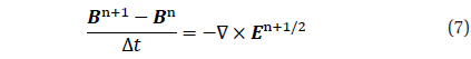
Next, we solve Faraday’s induction equation, Eq. (2), using the lead-frog scheme to advance the magnetic field in time delineated by the following discretized equation.

Using the electric and magnetic fields we solve the relativistic Lorentz force equation, Eq. (5). As a result of using the leap-frog scheme, as Eq.(7), the electric field and the magnetic field are determined at different times: the electric field at (n + 1) Δt, and the magnetic field at at (n + 1)Δt. To obtain the values at the same time, (n + 1)Δt, we average the magnetic fields at nΔt and (n + 1)Δt. To solve the relativistic Lorentz (Birdsall & Langdon 2004).

Particles are then moved to new positions by sloving the following equation:

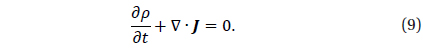
Finally, we solve the Ampère-Maxwell equation, Eq. (1), using the current density and the magnetic field to advance the electric field in time. The estimation of the current density is complicated and many methods have been suggested to correctly calculate the current density (Villasenor & Buneman 1992, Esirkepov 2001, Umeda et al. 2003). Generally, wwe can calculate the current density as J = ∑_in_iq_iv_i, However, this does not satisfy the charge conservation in discrete grid systems. To satisfy the charge conservation, we have to correct the electric field using some method, or the electric field must have a divergence-free part only. Alternatively, various methods have been suggested to satisfy the charge continuity equation as given below:

To slove the Poisson equation and calculate the current densiy it is necessary to estimate the charge density onthe grids from particle distributions The contribution of a particle to the charge density on a grid is determined by using shape functions. In this code, we use second-order shape function in two-dimensions, given as follows:

Using the second-order shape function, one particle contributes to 9 adjacent grids. The higher-order shape function has the advantage of reducing numerical errors, but at the cost large calculation time.

The time integration of all the differential equations is achieved by using the leap-frog scheme, as mentioned above. To carry out the leap-frog scheme, all the variables that have time dependence are divided into the variables defined at the full-integer time step, (n + 1)nΔt. For example, the magnetic field, current density, and velocity are defined at the full-integer time step while the electric field and position at the half-integer time step.

For the differentiation in space we use the centered difference scheme. In this scheme, the variables are defined either at a full-integer grid or at a half-integer grid, which is called a staggered grid system. For example, the charge density, electrostatic potential, and E_z are defined at the fullinteger grid both in the x- and y-directions. On the other hand, E_x and B_y are defined at the half-integer grid in the x-direction and the full-integer grid in the y-direction, E_y and B_x are defined at the full-integer grid in the x-direction and the half-integer grid in the y-direction, and B_z is defined at the half-integer grid both in the x- and y-directions.

To test the developed code, we simulated the electron two-stream instability and the whistler instability using the same parameters as described in previously reported papers and compared the results with those of the previous papers.

First, we simulated the electron two-stream instability with the parameters used by Umeda (2004). In this simulation, the length is normalized by the Debye length, λ_De, and time by the electron plasma frequency, w_pe, satisfying λ_De = v_the / w_pe, where is the electron thermal speed. The system size is L_X × L_Y = 256λ_De × 256λ_De, and the number of grids is N_X × N_Y = 256 × 256, which makes the grid size Δx = Δy = 1.0λ_De. The number of particles in a cell is set to be 128 for the electrons and protons, respectively. The ratio of the electron plasma frequency and the electron gyro-frequency is set to be w_pe / Ω_pe, and the electron thermal velocity v_the = 0.05c. The background magnetic field is oriented in the X-direction , and the magnitude of the magnetic field, B₀, is determined by the electron gyro-frequency. Boundary conditions are set to be periodic in both the X- and Y-directions.

To excite the electron two-stream instability, electron beams drifting oppositely to each other were initially injected uniformly throughout the simulation domain. The densities of the two beams were the same. The bulk speeds of the beams were ±2v_the, which makes the relative speed between the beams 4v_the. To make the simulation conditions identical with Umeda (2004), we assumed that protons are immobile. This assumption is acceptable because the mass of protons is much larger than that of electrons and the electron two-stream instability develops in the time scale of electrons.

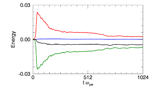
The simulation results are presented in Figs. 1 and 2. Fig. 1 shows the temporal variations of the electric field energy density, 2>, magnetic field energy density, 2>, kinetic energy density, 2/2>, and total energy density averaged over the whole simulation domain. Because the two-stream instability is an electrostatic instability, the electric field energy rapidly increases as the instability grows while the magnetic field energy remains almost constant. The increased electric field energy comes from the kinetic energy of particles, which decreases in coincidence with the increase of the electric field energy. This is consistent with the theory of the two-stream instabilities. After the electric field energy reached the maximum, it gradually decreased while the kinetic energy increased.

The drastic variations of energies in the growth phase of the instability produced numerical errors, which caused a loss of the total energy. However, during gradual variations of energies, the total energy was well conserved. In comparison with the results of Umeda (2004), the variations of the energies are similar except for that in the case of Umeda (2004) the total energy density gradually decreased even after the decrease in the rapid growth phase.

Fig. 2 shows the distribution of the electrostatic potential at w_pet = 60, w_pet = 260, and w_pet = 1020. Because the two electron beams drift oppositely along the background magnetic field, the electrostatic waves propagate parallel to B₀ producing sinusoidal oscillations of the potential (Fig. 2a), which are represented as electron holes in the phase space. After the instability reached saturation at w_pet ~ 60, the wave structures or electron holes merged together until there remained only one structure. In comparison with the results of Umeda (2004), the wave structures are very similar in the early development stage in Fig. 2a. In Figs. 2b and 2c, however, the merging of the structures was slightly faster in our results than in Umeda (2004), which might be related to the difference in the variations of the energies.

Next, we followed the initial configurations of Run 3 in Gary et al. (2011), who investigated the electron temperature-driven whistler instability using their PIC code. The simulation system is normalized by λ_e in space and w_pe in time, satisfying λ_e = c / w_pe, where λ_e is the electron inertial length. The system size is L_X × L_Y = 12.85λ_e × 12.85λ_e, the number of grids is N_X × N_Y = 64 × 64, and the number of particles is set to be 9600 particles in a cell for each of the electrons and protons. The ratio of electron plasma frequency and electron gyro-frequency is set to be w_pe / Ω_ce = 4.0, where Ω_ce = eB / m_e is the electron gyro-frequency. Ions are assumed to be an immobile background as in the previous case. Periodic boundary conditions are used for both the x- and y-directions. The background magnetic field is applied along the x-direction, .

To excite the instability, the electron temperature anisotropy in the perpendicular and parallel directions to the background magnetic field is applied as .T_⊥e/ T_||e, and the parallel plasma beta of electrons is given as β_||e = 0.01.

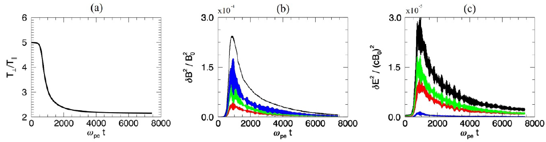
Fig. 3. shows the temporal variations of the temperature anisotropy, T_⊥e/ T_||e, magnetic energy density, , and electric energy density, δE² / (cB₀)², of the fluctuations. As the instaility grew, the temperature anisotropy decreased rapidly while the electric and magnetic energy densities increased. The kinetic energy density decreased in coincience (not shown). Note that the magnetic energy density is an order of magnitude larger than the electric energy density. The growth of the B_z component was dominant, which corresponds to the growth of the E_x and E_y components. In comparison with results of Gary et al. (2011), all the variations are almost the same except for that our results evolve slightly faster. It should be noted that time was normalized by the electron cyclotron frequency in Gary et al. (2011), but in our simulation it was normalized by the electron plasma frequency. The ration between the frequencies is ω_pe / |Ω_e| = 4, where ω_pe and Ω_e are the electron plasma frequency and the cyclotron frequency, respectively.

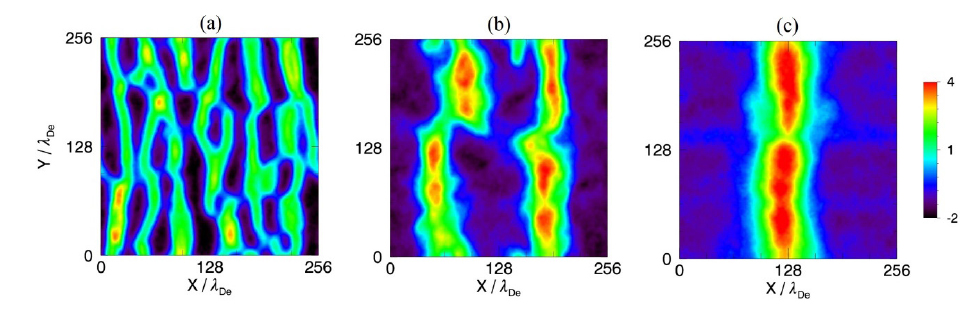
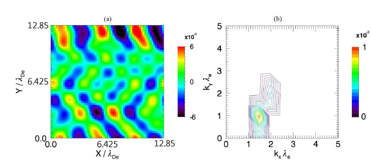
Fig. 4. shows the distributions B_z(x,y) in the configuration space and B_z(k_||, k_⊥) in the k-space at ω_pet = 740 when the instability is close to saturation. It is seen that the whistler waves propagate obliquely. The spatial distribution of the B_z component and the propagation characteristics of the whistler waves in our simulation results are almost identical with those of Gary et al. (2011). The only difference is that the wave number, k, of our results is slightly smaller than that of Gary et al. (2011), which implies that the wavelength of the generated whistler waves is slightly longer in our results.

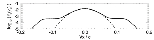
Fig. 5 shows the parallel velocity distribution of electrons at the initial and final stages of the simulation. As a result of the instability, suprathermal electrons were generated in the range of 4 ≤ |v_||e|/v_the ≤ 6 in the direction parallel to the background magnetic field. The generation of suprathermal electrons in the parallel direction reduced the temperature anisotropy T_⊥e/ T_||e. However, it should be noted that the temperature is not well defined for the distribution seen in Fig. 5 because the distribution is a non-Maxwellian distribution consisting of the core and suprathermal components. According to Gary et al. (2011), the suprathermal electrons were produced by the acceleration by the parallel component of the electric field through Landau resonance. The velocity distribution of electrons is also consistent with that of Gray et al. (2011).

In this paper, we briefly introduced the 2.5-dimensional relativistic electromagnetic PIC code that we have developed and tested the performance of the code by comparing the results obtained from the code with those of two widely used codes reported in previous studies.

First, we performed a simulation of the electron two-stream instability to test the availability of handling the plasma dynamics in electrostatic phenomena. Our simulation results captured most of the physical features presented in Umeda (2004) except that merging of the electron holes in the relaxation phase took place slightly faster in our simulation. Note that both codes suffered similar numerical errors during the rapid growth of the instability. The loss of the total energy appears to be related with numerical diffusion and our code has slightly larger numerical diffusion than Umeda’s. This also appears in the merging rate of the electron holes, which is faster in our results than those of Umeda. Thus, we should be cautious for unphysical loss or gain of energies when a process occurs rapidly. However, the loss or gain of energies was not significant enough to affect the main physical processes.

Next, we performed a simulation of the whistler instability driven by electron temperature anisotropy to test for handling the plasma dynamics in electromagnetic phenomena. In this case, our simulation successfully produced the whistler instability and the results of our simulation were also almost identical with those of Gary et al. (2011). A slight difference was found in the wavelength of the generated whistler waves. However, this did not substantially affect the main features of the instability.

In conclusion, the PIC code we have developed successfully reported in previous studies for both electrostatic and electromagnetic phenomena. We will further improve the code in future studies to reduce the numerical errors by applying higher-order shape functions or by implementing other numerical schemes.