Thunderclouds are tropospheric sources of intense electrostatic fields and electromagnetic radiation. It is known that lightning-associated electric fields penetrate into the ionosphere; they have been observed in the E and F regions as transient electric fields with a typical duration of 10-20 ms and a magnitude of 1-50 mV/m (e.g., Kelley et al. 1985, 1990; Vlasov & Kelley 2009). According to the theoretical model of global atmospheric electricity developed by Hays & Roble (1979), the African array of multiple thunderclouds is responsible for the steady state electrostatic field of ~300 μV/m at ionospheric altitudes for nighttime conditions. The calculations by Park & Dejnakarintra (1973) showed that an isolated giant thundercloud could produce electrostatic fields of ~700 μV/m in the nighttime midlatitude ionosphere. However, Park & Dejnakarintra (1973) neglected the ionospheric Pedersen conductivity above 150 km. The purpose of this study is to theoretically examine the mapping of electrostatic fields of coulomb charges of an individual thundercloud into the midlatitude ionosphere, taking into account the height-integrated Pedersen conductivities of both hemispheres.

In the simplest thundercloud model, the electrical structure of a thundercloud is represented by two volume Coulomb charges of the same absolute value Q but opposite signs, with a positive charge in the upper part of the thundercloud and a negative charge in the lower part of the thundercloud (e.g., Chalmers 1967). Typical thunderclouds extend from 2-3 km to 8-12 km in altitude, and so-called giant thunderclouds extend above an altitude of 20 km (e.g., Uman 1969; Weisberg 1976). The magnitude of Q is estimated to range from 5 to 25 coulombs for the typical thunderclouds, whereas in giant thunderclouds, Q may exceed 50 coulombs (e.g., Malan 1963; Kasemir 1965).

We use a cylindrical coordinate system (r, φ, z), in which the origin is placed at the earth’s surface and the z axis points upward and passes through the centers of thundercloud positive and negative volume charges. The mapping of thundercloud electrostatic field into the ionosphere is studied following a similar formalism to that used by Park & Dejnakarintra (1973). In the steady state case, the electrostatic field distribution above the thundercloud is described by the following equations:

where J is the electric current density, σ is the electrical conductivity tensor, and E and Φ are the electrostatic field and potential, respectively. If we assume that the geomagnetic field B is vertical and the electrical conductivity tensor depends only on z, the following equation for the electrostatic potential Φ cna be obtained from (1), (2), and (3) :

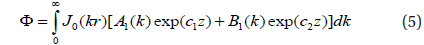
where σ_p is the Pedersen conductivity and σ₀ is the specific conductivity. The atmospheric conductivity below 70 km is isotropic since drifts of charged particles are not affected by the geomagnetic field. Equation (4) can be solved analytically if the conductivities σ₀ and σ_p are exponential functions of z. In the case of isotropic conductivity (setting σ₀=σ_p=b exp(z/h), where b and h are constants), we obtain

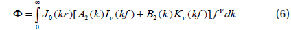
where J₀ is the zero-order Bessel function of the first kind, A₁ and B₁ are coefficients, and c₁= -l/(2h) -[l/(4h²)+k²]^1/2, c₂= -l/(2h) + [l/(4h²)+k²]^1/2. For the anisotropic region, where we let σ₀ = b₀ exp(z/h₀) and σ_p = b_p exp(z/h_p), the solution to Equation (4) is

where J_ν and K_ν are the ν-order modified Bessel functions of the first and the second kind, respectively, and A₂ and B₂ are coefficients, ν=h_p/(h_p-h₀), f=2νh₀(b_p/b₀)^1/2 exp[-z(2 νh₀)]. The coefficients A₁, B₁, A₂, and B₂ are determined from the boundary conditions.

The electrostatic field components are given by

Since the geomagnetic field B is assumed to be vertical, E_r is perpendicular to B, while E_z is parallel to B.

Above 90 km, the geomagnetic field lines are practically equipotential because the geomagnetic field aligned conductivity σ₀ is much higher than the transverse conductivity σ_p. It allows us to consider the ionoshperic region above 90 km as a thin conducting layer with a geomagnetic field line integrated Pedersen conductivity Σ_p, and the continuity equation of electric current at z=90 km takes the following form:

where ▽_⊥ denotes the gradient operator in the two dimensions transverse to B, and the factor 2 before Σ_p accounts for a contribution of the Pedersen conductivity of the magnetically conjugate ionosphere. Equation (9) is explicitly expressed as

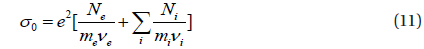
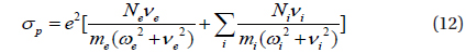
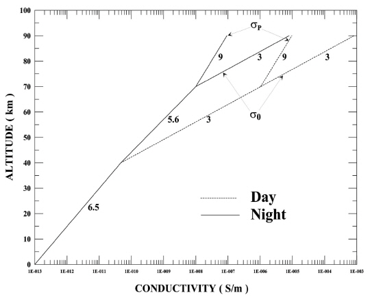
We use the conductivity model as shown in Fig. 1. Below 70 km, the conductivity is isotropic and varies exponentially with z as σ₀₁=σ_p1=b₁ exp(z/h₁) from 0 to 40 km, and as σ₀₂=σ_p2=b₂[exp(z-z₁)/h₂] from 40 to 70 km (where z₁ = 40 km) with the values of b_1,2 and h_1,2 to approximately fit the atmospheric conductivity models by Cold & Pierce (1965) below 40 km and by Swider (1988) from 40 to 70 km. In the anisotropic region between 70 and 90 km, σ₀, and σ_p are exponentially extrapolated from 70 km to their equinoctial midday and midnight values at z=90 km. At z ≥ 90 km, the conductivities are found from

where subscripts e and i denote electrons and the ith ion species, N_e and N_i are the electron and ion densities, e is the electron charge, m_e and m_i are the electron and ion masses, ν_e and ν_i are the electron and ion momentum transfer collision frequencies, and ω_e and ω_i are the electron and ion gyrofrequencies, respectively. The frequencies ν_e and ν_i are from Schunk (1988). The required input parameters are taken from the empirical ionospheric model IRI-2012 (http://omniweb.gsfc.nasa.gov/vitmo/iri2012_vitmo.html) and the neutral atmosphere model NRLMSIS-00 (http://ccmc.gsfc.nasa.gov/modelweb/models/nrlmsise00.php).

Our calculations show that during solar minimum, in Equinox, the magnitude of Ʃ_p at middle latitudes is commonly in the ranges of 5.0-8.0 S and 0.1-0.2 S for day and night, respectively. However, the nighttime Ʃ_p can be as low as 0.05 S. Under solar maximum conditions, Ʃ_p is several times larger than in solar minimum.

To compute the electrostatic potential above the thundercloud from (5) and (6), we impose the following boundary conditions:

1. Φ=(Q/4πε0)[(r2+(zb-hp )2)-1/2-(r2+(zb-hn )2)-1/2 ] at z=zb 2. Φ is continuous at z=40 km 3. σ0 ∂Φ/∂z=2Ʃp (∂2Φ/∂r2+1/r ∂Φ/∂r) at z=90 km

where ε₀ is the vacuum permittivity, z_b is the altitude of the plane setting directly above the thundercloud top, and h_p and h_n are the altitudes of positive and negative charge centers of the thundercloud, respectively. The first boundary condition follows from the accepted electrical model of the thundercloud. We assume that the thundercloud does not affect the atmospheric conductivity at z≥z_b.

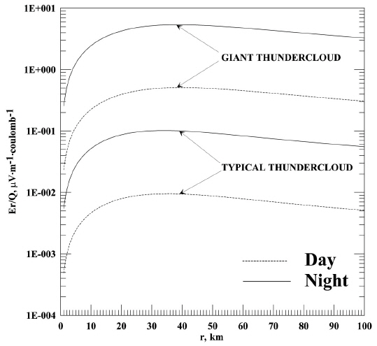
Fig. 2 shows the computed electrostatic field component E_r normalized to Q as a function of r in the nighttime and daytime midlatitude ionosphere at z≥90 km for the typical thundercloud (z_b=10 km, h_n=3 km, h_p=8 km) and for the giant thundercloud (z_b=20 km, h_n=5 km, h_p=17 km). Solar minimum conditions are considered with Ʃ _p=0.05 S at night and Ʃ _p=5.0 S by day. All curves show similar behavior, attaining first a maximum and then revealing a gradual lowering. At night, the thundercloud electrostatic field is transmitted into the ionosphere much better than during the daytime. For a typical thundercloud, Er reaches its nighttime maximum value of ~2.6 μV/m (for Q=25 coulombs) at r~35 km. In the case of the giant thundercloud, the nighttime maximum magnitude of E_r is ~270 μV/m (for Q=50 coulombs) and r_max~40 km. The daytime maximum values of E_r are one order of magnitude less than their nighttime values. Thus, the steady state electrostatic fields associated with the individual typical thunderclouds have very small magnitudes at ionospheric altitudes. In the case of a giant thundercloud, E_r is two orders of magnitude larger. Note that Park & Dejnakarintra (1973) discovered that the maximum magnitude of the transverse electrostatic field produced in the nighttime midlatitude ionosphere by a giant thundercloud with Q=50 coulombs can be as large as ~700 μV/m, which is about 2.6 times more than in our estimate. This difference can mainly be attributed to the fact that Park & Dejnakarintra (1973) ignored the Pedersen conductivity above 150 km.

Our computations show that the geomagnetic field line integrated Pedersen conductivity of the ionosphere plays an important role in troposphere-ionosphere electrostatic coupling. Even for nighttime conditions in solar minimum, when the values of Ʃ _p are minimal, the electrostatic charges of the individual thundercloud can drive only small electrostatic fields at ionospheric altitudes.