The first discovery of an extrasolar planet in 1995 (Mayor & Queloz 1995) resulted in the opening of a completely new astronomical research area. However, detailed information about the planet, obtained via radial velocity measurements, was limited since only the minimum mass (among other parameters) could be inferred due to an unknown orbital inclination. The class of transiting extrasolar planets has changed this ambiguity. With the discovery of a transiting extrasolar planet (TEP) (Charbonneau et al. 2000; Henry et al. 2000) it became possible to determine the physical properties of the planet (mass and radius, among others) and its host star (limb darkening, effective temperature among others) when combined with spectroscopic observations. In principle, by obtaining precise measurements of these properties, one can distinguish whether a given TEP is a rocky terrestrial-size or gaseous Jupiter-size planet by inferring its absolute size and mass. Therefore, the accurate measurement of properties helps to constrain planet formation theories. One possible technique to obtain high-precision photometric light-curves is the use of the telescope defocus technique, and this method has been successfully applied in various studies, including Southworth et al. (2009).

This research presents results from our attempt to obtain precise light-curves of TEPs using a 0.6m telescope. In particular we present results in which the telescope was operated in-focus as well as out-of-focus. In Section 2, we outline the background of the defocus technique. In Section 3 we present our observations of seven TEPs observed since early 2012. A description of data reduction and light-curve modelling is given in Sections 4 and 5. Our results and analysis are given in Sections 6 and 7 followed by a conclusion in Section 8.

Traditional astronomical photometry aims to measure the brightness of a star with the telescope kept in focus, resulting in a well-defined point-spread function (PSF). This is usually desired when structural information is needed (e.g. star cluster observations to resolve individual stars) or when the observed star field is crowded, to avoid confusion due to overlapping PSFs. However, in certain situations the operation of the telescope in a defocused mode opens up the potential to achieve an increased signal-to-noise (S/N) ratio, resulting in a higher photometric precision. Nevertheless, the same noise processes are in operation whether the telescope is in-focus or de-focused. To obtain high-S/N measurements over an extended time period both instrumental and environmental effects are important to consider.

In general, several types of noise sources contribute to the overall error budget of a single measurement. The first class is random noise (also known as statistical, white or time-uncorrelated noise) and often referred to as Gaussian noise associated with Poisson counting statistics of photons. CCD read-out noise, CCD dark-current, shotnoise of the background as well as the target star are all referred to as random noise. In a special case, atmospheric scintillation noise is also of a random nature, but this also depends on other factors such as telescope aperture (see below for more details). To decrease white noise requires an increase in the photon counting statistics. The second class of noise source is of a systematic nature and harder to identify and/or quantify. Examples of systematics would be selecting aperture sizes for photometry or flat-fielding errors involving the positioning of the target star on the same pixels. Controlling the latter is ultimately linked with telescope pointing stability and involves how well the telescope is tracking over an extended time period. Also the choice of comparison stars for differential photometry is a potential source of systematic noise. Furthermore, the telescope optical alignment (astigmatism) and general telescope optics also are potential sources for introducing systematic noise.

Other noise sources include non-random noise (also known as red, 1/f or time-correlated noise) often (but not exclusively) associated with atmospheric extinction encountered at the beginning and/or end of a transit observation when the target star is observed through high air-mass. The final error source is related to the intrinsic variability of the star itself, such as star spots, flares and pulsations. All of these noise sources have the effect of deteriorating the photometric time-series measurements in one or another way, making it difficult to obtain a photometric precision of less than a milli-magnitude.

One key aspect of limiting the S/N ratio of a photometric measurement is the dynamic range of a CCD detector, which dictates the peak flux and thereby sets a natural upper limit on the exposure time for a telescope operated in an in-focus mode. CCD detectors with a higher dynamic range allow for a longer exposure time, thereby circumventing the danger of reaching the saturation limit. Ideally, in order to obtain a high signal to-noise (S/N) ratio plenty of photons are needed (otherwise achieved by using a large mirror aperture). The larger the photon counts the lower the Poisson noise. One practical way to allow for a longer exposure time without saturating the CCD is to spread the light over many pixels by defocusing the telescope. As a result the stellar PSF of the target (and all other stars in the same field) broadens and decreases the peak value of an exposed pixel.

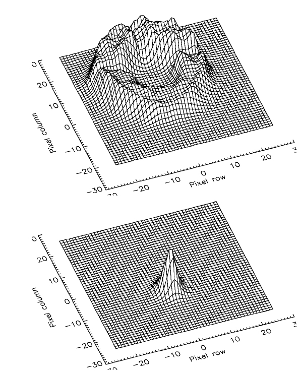
In Fig. 1, we show an example of two stars of fairly similar brightness, but defocused for the case of HATP22. Simply, in a defocus mode, the number of photons are distributed over a larger area of the CCD allowing a prolonged exposure and hence a stronger signal to build up and stand out from the baseline of combined noise sources.

However, there is a natural upper limit of exposure time (t_exp), which is determined by the single frame read-out time (t_ro) and the transit duration (t_dur), as follows

where N is the number of frames recorded during the transit. To characterise a planetary transit with a detailed modeling process the light-curve sampling has to be sufficiently high in order to ensure enough measurements. As a rule of thumg we aim to obtain N = 30 to 40 measurements during a given transit event, resulting in 4 to 6 measurements of the ingress and egress phase.

Several advantages and disadvantages of the defocus technique contribute to either a decrease or increase in the S/N ratio. The effect of variable atmospheric seeing and local temperature changes are less important for observations with a broad PSF. However, high atmospheric transparency is still desirable. Distributing the photons over many pixels also has the effect of decreasing the photometric noise due to intrinsic CCD pixel-to- pixel response variations. The total flatfield noise contributio within a larger signal aperture (contribution of each pixel added in quadrature) is lower when compared to a similar in-focus measurement. In essence, the flatfield error of the final photometric measurement should average out using a larger number of independent pixels due to its random nature.

One technical possibility by which one can increase the number of pixels is to operate the CCD in one-by-one binning. When the maximum number of pixels are requested, the readout time in single-pixel binning mode is maximised. Forming super pixels via two-by-two (or higher) binning can decrease the read-out time.

However, a disadvantage of defocus photometry is the contribution of CCD read-out noise. The more pixels that are exposed the larger the total read-out noise will be on a given measurement. In addition, the contribution of background noise in the broadened PSF will also decrease the photometric S/N.

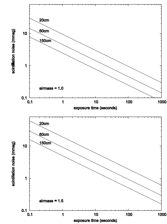
A positive effect of a prolonged exposure for a small aperture telescope is the beating of scintillation noise. Scintillation is caused by the refraction of starlight (twinkle) by turbulent cells in the atmosphere. The effect introduces a time-varying fluctuation in the star’s brightness. Its effect is largest for telescopes with small mirror diameters and short exposure times. Therefore, scintillation will set a lower-limit of the photometric precision obtained from a small-aperture telescope. Young (1967) was the first to model the effect of scintillation for bright stars. Using the expression given in Hartman et al. (2005) we have examined the dependence of scintillation noise on telescope aperture, air-mass, telescope height and exposure time. In Fig. 2, we plot the scintillation noise (in milli-magnitude) as a function of exposure time for three different telescope apertures located at 80 m above sea level. The top panel shows the relationship for air-mass=1.0 and the lower panel for air-mass= 1.5. In general, the scintillation noise decreases with either increasing telescope aperture or increasing exposure time at a given air-mass. Considering a 60 cm telescope, at unit air-mass and integrating for 250 seconds, the scatter per data point expected from scintillation is below 0.3 mmag. At air-mass 1.5 this limit increases to 0.6 mmag-more than sufficient to record transits depths of 1 - 2% with good precision. However, scintillation imposes a lower limit which is achievable for only bright stars.

All observations presented in this work were carried out using the 0.6 m telescope (hereafter CbNUOJ) located in Jincheon at an altitude of 87 m above sea-level. The telescope was installed by the Korea Astronomy and Space Science Institute (KASI) and is operated by Chungbuk National University Observatory, Republic of Korea. The telescope optics follow the Richey-Chrétien design, attached to an equatorial mount. Telescope tracking is performed via a servo motor control. More details of this telescope were described by Kim et al. (2014).

During the observing period the telescope was equipped with two different CCD imagers located at the Cassegrain f/2.92 prime focus and installed by the Korea Astronomy and Space Science Institute (KASI). Initially we used the 1530 x 1020 pixel SBIG ST-8XE which was later replaced (currently installed) by the more advanced 4096 x 4096 pixel SBIG STX-16083 CCD camera. The former camera had a field of view of 27´× 18´and the current camera provides a field of view of 72´×72´. Both cameras had a pixel scale of 1.05 arcsec/pixel. Single Johnson/Cousins UBVRI filters are available via an electronic filter wheel system. For most of our observations we used the Cousins R-filter. In some observations we experimented with clear filters. The large field of view in the current instrumental setup is ideal for differential photometry when carrying out ensemble photometry analysis (Everett & Howell 2001). Both cameras are cooled electronically.

Unbinned CCD read-out time for the ST-8XE was about 10 seconds while for the STX-16083 camera it was around 16 seconds. The two relatively short read- out times are favourable for high-cadence transit photometry and allowed us to stay on target for a larger fraction of time for photon collection. Another benefit of short read-out times is a smaller contribution to the noise budget due to read-out noise imposed on a single frame, as the high photon counts will dominate for defocus measurements.

In the beginning (2012 season using the ST-8 camera), we followed a strategy where we changed the exposure time during a given night according to weather conditions. Later we abandoned this strategy and kept the exposure time fixed for consistency of the recorded data. In our experience even thin clouds will usually have a dramatic temporal effect on the sampled light-curve when trying to aim for a mean ~1 mmag photometric precision over 3 to 4 hours. Changing exposure times by a few percent did not have a significant impact on the signal-to-noise ratio and our goal was to ensure a well-sampled light curve.

All observations were carried out with the cameras operated in unbinned mode providing a maximum number of pixels favourable for defocus photometry. Prior to the defocus observations we aimed to obtain 2-3 in-focus images in order to identify any nearby companions. The average seeing at CbNUOJ is around 2 arcsec.

Calibration frames (bias and skyflats) were obtained for each night using an appropriate filter. We carried out tests in which the science images were either calibrated or kept in their original form. We report the results from those experiment in the next section. An observation log is given in Table 1. Details of the observed host stars are given in Table 2.

We used the DEFOT data reduction pipeline outlined in Southworth et al. (2009). The software is written in IDL and makes use of the NASA IDL astronomy library package astrolib. The method of obtaining photometric measurements is by following the algorithm described in the DAOPHOT photometry package. Aperture photometry is done using the astrolib/aper routine. UTC (Coordinated Universal Time) time stamps in the format YYYY-MM-DD/HH-MM-SS are obtained from each image FITS header. Actual times for a single photometric measurement were taken to be the mid-exposure time. To convert to Barycentric Julian Date (BJD) in the Barycentric Dynamical Time (TDB) standard we used the utc2bjd.pro conversion routine of Eastman et al. (2010). BJD time stamps expressed in the TDB standard are particularly useful when searching for transit timing variations (TTV).

Apertures for the inner and background annulus were fixed (but their optimum values determined from experimentation) in all frames for each data set. We noticed a significant frame-to-frame shift due to tracking imperfections of the telescope. To ensure that the apertures were following the selected stars (target and comparison) we made use of the image registration cross-correlation algorithm available in the DEFOT package. For each program image a summed pixel row and pixel column intensity profile is calculated and compared with the same profile of a reference frame. A least squares high-order polynomial fit is then performed to calculate any shifts and a given frame is then corrected accordingly in order to match the reference frame. The downside of the package is that only a single aperture for the three annuli is applied to all stars. In practice this limits the selection of comparison stars to those similar in brightness (and hence angular extend on the CCD) with the target. From experimentation we used apertures that yielded the smallest root-mean-square (RMS) scatter around a best-fit model (see next section). Table 3 gives an overview of the various apertures used for each target.

Comparison stars were checked for internal variability and none were found for the selected stars. The DEFOT package allows ensemble differential photometry to be carried out using weighted flux summation. This procedure minimises the overall Poisson noise while also avoiding distortion in the transit light curve. More details of this procedure can be found in Southworth et al. (2009) and Everett & Howell (2001).

Long-term trends over the observing window were removed using a polynomial fit to out-of-transit data. The resulting light curve was then normalized to zero differential magnitude. In all normalisations we applied a first-order polynomial fit. Higher-order terms would have the potential of introducing artificial distortions to the transit light curve.

In some cases we noticed obvious data outliers, most likely due to passing thin clouds. These were removed prior to our photometric analysis. To find stable comparison stars we selected all suitable stars and carried out a first selection by eye. Then a subset of stable stars (4-15) were included in the final photometric analysis. To find optimum apertures we varied the three radii in a systematic way. For each experiment we found a best-fit solution with associated RMS scatter of the residuals. Radii resulting in a least scatter were chosen. These experiments were done using raw science frames. Using the most optimal apertures we also calibrated (bias subtraction and flatfielding) the science frames to determine any difference in RMS. In some cases we found that a calibration resulted in a slight improvement in the photometry, while in other cases we found no improve-ment.

Light-curves of all transiting planets were modelled using the JKTEBOP_V25 least-squares minimisation code Southworth (2008); Southworth et al. (2009). The code models the light curve of detached eclipsing binary stars using biaxial spheroids. Fundamental parameters (star and planet are referred to with subscripts A and b, respectively) describing the light-curve of transiting planets are the orbital period P, the time of minimum light T₀ (or ephemeris epoch when modelling multiple light-curves simultaneously), the fractional radii of the star (r_A = R_A/a where a is the orbital semi-major axis) and planet (r_b = R_b/a), the orbital inclination (i_b) and limb-darkening coefficients. In practice, the parameters r_A and r_b are parameterised as their sum (r_A + r_b) and ratio (k = r_b/r_A).

In all modelling work we kept the radii sum, radii ratio, orbital inclination, the time of minimum light and the scale factor (normalised flux level) freely adjustable. Since this work presents transit data of a single event for a given planet we did not fit for the orbital period and kept it fixed. Stellar limb-darkening was implemented in JKTEBOP in the form of several parametric laws. A linear or quadratic limbdarkening law introduced another one or two parameters. Initial guesses of known quantities have been obtained from the respective discovery papers for each system.

When using JKTEBOP_V25 in its simplest form (TASK3) the parameter uncertainties are obtained from the bestfit covariance matrix. Therefore they are formal (and probably too optimistic) errors. More proper parameter uncertainties are obtained through the implementation of bootstrapping, Monte-Carlo and residual- permutation (RP) algorithms. To obtain robust parameter uncertainties for light-curves with correlated red noise the RP algorithm is the most suitable, and available via TASK 9.

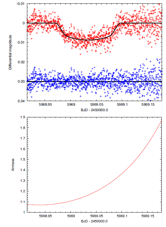
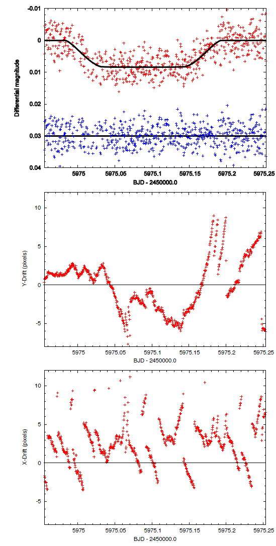
Our first few test observations with the telescope in focus aimed at recording transit light-curves of XO5 (Burke et al. 2008), XO3 (Johns-Krull et al. 2008) and XO4 (McCullough et al. 2008). The resulting light- curves are shown in Fig. 3, Fig. 4 and Fig. 5, respectively. In all three cases the transit is clearly visible. The photometric point-to-point scatter is no less than ~3 mmag with maximum exposure times ranging from 105 seconds for XO5 (V = 12.1 mag) to 12 seconds for XO3 (V = 9.9 mag). Short exposure times result in a high sampling cadence. The residuals in each plot all show some degree of systematic effects indicating that correlated (red) noise is the most dominant error source. In all cases the photometric precision is too low for a sufficient characterisation of the transit. The derived planet parameters have a large uncertainty. Nevertheless we modelled the light-curves in order to obtain an estimate of the mid-transit time. Limb-darkening treatment is not meaningful since no such effect is readily apparent in the time-series photometry. Errorbars per observation have been omitted in the figures to highlight some details concerning our observing strategy, sky condition and telescope tracking properties.

In Fig. 3, we also plot the exposure time used during the observing window. Depending on sky condition we varied the exposure between 75 seconds and 110 seconds. After BJD 2,455,968.15 the scatter systematically shifts upwards in the differential magnitude plot. This coincides with a period of time where the exposure time was chosen to be minimal, demonstrating that decrease in exposure time deteriorates the photometric precision. This finding motivated us to stick to a constant exposure time during the course of observation, resulting in a homogeneous data set.

In Fig. 4, we chose to plot the air-mass during the XO3 transit. We demonstrate that observing through a relatively high air-mass (>1.45) results in a significant increase in photometric scatter, most likely due to a larger scintillation noise. To obtain high-precision photometry of a transiting planet one should aim to observe through as low air-mass as possible. This requirement would exclude targets located on more southern latitudes

A last characteristic is concerned with the pointing ability of the telescope itself. The cross-correlation algorithm as implemented in DEFOT for image registration records the number of pixels by which each program image was shifted in order to match the reference image. In Fig. 5, we plot the telescopic x- and y-drift measured in pixels during the XO4 transit observation. The x-drift corresponds to ± rightascension while y- drift is ± declination. In both directions the maximum drift is around 10 pixels (10.5 arcseconds). While the y-drift appears to be of a continuous nature the x-drift occurs in jumps. Pointing imperfections can either be due to a lag in the motor drives/friction-disk, inaccurate encoder and/or software control. The ability to keep the target on the same pixels during the transit observations contributes to minimising flatfielding errors. As an example the recently commissioned K2 mission (Kepler space telescope extended mission) will have its photometric precision decreased significantly (compared to the original Kepler mission) due to decreased pointing accuracy.

In order to obtain high-precision photometric measurements of a transiting planet we then carried out tests with long exposure times per observation frame. A significant amount of telescope defocus would be required for the much brighter targets to ensure that ADU counts would be in the linear regime of the CCD. We obtained four light-curves of four different systems on four different nights. Three of the recorded light-curves make use of the new ST-16083 CCD camera.

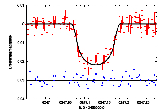
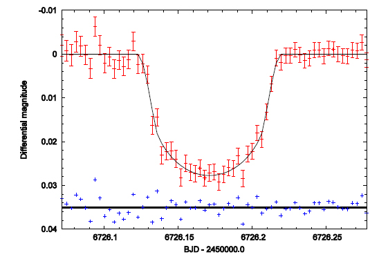
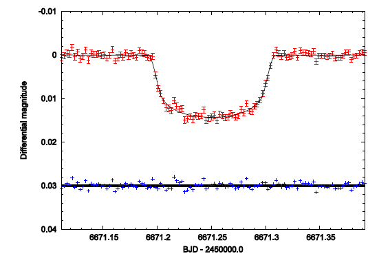
In Fig. 6 to Fig. 9, we show the light-curves of HATP25 (Quinn et al. 2012), HATP9 (Shporer et al. 2009), HATP22 (Bakos et al. 2011), HATP12 (Hartman et al. 2009). Light-curves of HATP12 were previously recorded several times using the Korean 1 m optical telescope at Mt. Lemmon Optical Astronomy Observatory (LOAO), Arizona, USA Lee et al. (2012). All light-curves were observed through a Cousins R-filter. The sampling frequency is now due to a longer exposure time. Exposure times of over 3 minutes have been used on average. The effect is immediate and we see a significant increase in photometric precision compared to our first test observations (see previous section). Using a fixed exposure time of 260s we achieved a RMS scatter of ~1.85 mmag for the faintest host star (HATP12, V = 12.8 mag). A remarkable RMS scatter of 0.70 mmag was obtained for the brightest target HATP22 (V = 9.8 mag).

Quadratic limb-darkening coefficients for Cousin R-filter were obtained using the JKTLD code which outputs theoretically calculated limb-darkening strengths for a variety of parametric laws. The coefficients are calculated from bilinear interpolation (in effective temperature and surface gravity) from published tables calculated from stellar model atmospheres. In this work we obtained the coefficients for the quadratic limb- darkening law from tables published in Claret et al. (2000). In all cases we assumed the metallicity of the host-star to be zero and the atmospheric micro variability parameters were set to unity. Using nominal published values for Tef f , log g, [Fe/H] and vmic does not allow one to determine suitable coefficients.

JKTEBOP allows parameter uncertainties to be obtained from two different methods depending on the noise character in the data set. If the observational noise is time-correlated (red noise or covariant noise, see eventually Gillon et al. (2009)) then TASK9 is recommended: it makes use of the residual-permutation (a variant of prayer-bead) algorithm. If the noise is Gaussian or white noise then a standard Monte-Carlo algorithm is implemented via TASK8. The former method requires the computation of n shifted fits where n is the number of data points. The latter method requires a larger number of simulations and we used 10,000 experiments to obtain parameter uncertainties from TASK8.

The remaining question is how to judge whether a given data set contains red or white noise. One method is to calculate the power spectral density of the photometric time-series or its residuals from a best-fit solution. If the observations have a high content of time-correlated (red) noise then the power spectrum of the timer-series will exhibit a 1/frequency dependence: most power at low frequencies. To test this behaviour we calculated the power spectrum of a single HATP16 transit observed with the 1 m reflector at Mt. Lemmon Optical Astronomy Observatory. Figure 10 shows the observed transit along with a bestfit solution. Systematic trends in the residuals are clearly visible during the observing window. The lower panel shows the power spectrum computed from a Lomb-Scargle algorithm as implemented in the PERIOD04 software package (Lenz & Breger 2005) with a clear 1/frequency trend pointing towards a significant amount of correlated noise (also visible in the residual plot in Fig. 10).

We have calculated power spectra for the four planetary transits obtained with the CbNUOJ telescope and display the results in Figure 11. In all cases (with the HATP25 transit as a possible exception with a marginal content of red noise) the power spectrum is flat (certainly no 1/frequency dependency) and hence no time-correlated red noise is present in these data sets. We therefore decided to use JKTEBOPs TASK8 for all transit observations to estimate parameter uncertainties. Since HATP25 could have red noise components, in that case we also estimated parameter uncertainties using TASK9.

For HATP25, we first fitted for the two limb-darkening coefficients separately. We found that the data does not allow a simultaneous fitting for the coefficients and found that the sum of final coefficients was larger than unity(implying an unphysical brightening at the host-star limb). We therefore decided to fix those parameters at their theoretical values, as shown in Table 4. The final best-fit parameters for the HATP25 transit is shown in Table 5. Since we estimated parameter uncertainties using TASK8 and TASK9 we can now judge that some amount of timecorrelated red noise is present for that dataset. The errors obtained from TASK9 are consistently larger than for TASK8.

For HATP09, we also fitted for the two limb-darkening coefficients separately, but encountered the same problem as found with HATP25 (i.e unphysical limb-darkening coefficients). We then set the two linear and quadratic terms to their tabulated values as obtained from JKTLD and fixed those parameters. In this case we found that the inclination was kept artificially at 89.96 degrees to ensure numerical stability of the minimisation algorithm. However, the best-fit inclination in the discovery paper Shporer et al. (2009) found an inclination of 86.5 degrees. We therefore decided to model the light-curve with a linear limb-darkening law using 0.5588 for the linear term as obtained from Claret et al. (2000). The resulting best-fit parameters along with uncertainties are listed in Table 5.

For HATP22, we judged that the amount of correlated red noise was minimal. We therefore used TASK8 (Monte-Carlo) to find parameter uncertainties based on 5000 simulations. The photometric precision is of high quality allowing us to fit for the two limb-darkening coefficients simultaneously without producing unphysical results. We also carried out fits where one of the parameters was held fixed. All three cases were consistent within the quoted uncertainties. The timing uncertainty for this light-curve was the smallest with around ±17 seconds. A close inspection of the HATP22 light-curve shows some systematic brightening at around BJD 2,456,671.215 and could be due to a star spot (Nutzman et al. 2011; Oshagh et al. 2013). However, this feature is also present in all the adopted comparison stars and is hence attributed to a short-term atmospheric change likely due to thin clouds.

For HATP12, we again inferred parameter uncertainties using TASK9. Also in this case we judged the errors to be dominated by correlated noise, especially prior to planetary ingress. We used a quadratic limb-darkening law with initial guess, obtained from Claret et al. (2000) and listed in Table 4. Both parameters were kept freely adjustable during the initial fitting process and we did not encounter unphysical results. The final best-fit parameters along with their uncertainties are shown in Table 5.

We have presented first results from follow-up observations of several transiting planets using the CbNUOJ 0.6 m telescope. In this study, we recorded light-curves using in-focus as well as defocused telescope settings. We qualitatively described various photometric noise sources and their effects when operating the telescope in a defocus mode. In particular we have outlined the advantage of defocused observations and demonstrated the ability to achieve a precision of RMS ~1 milli-magnitude over a timescale of several hours. We believe the precision can be explained by three factors: 1) long integration time (enabling the collection of many photons); 2) control of systematic noise sources due to good pointing precision by stable telescope tracking (keeping the tar- get star on roughly the same pixels) and; 3) beating of scintillation noise (as a side-effect of long exposure times) which otherwise would be significant for a 0.6 m telescope using exposure times of a few tenth of seconds when operating in the in-focus mode.

We demonstrated that the telescope is well suited for follow-up observations of suspected transit signals from discovery surveys such as Qatar, HAT, WASP and similar on-going projects. However, target stars with possible planets have to be bright, with a limiting magnitude of around V = 13~14 (depending also on the transit depth). For bright host stars with V ~10 a remarkable photometric precision of RMS~0.70 milli-magnitude was demonstrated for HATP22. This precision is high enough to determine physical properties of the planet with errors of a few percent. Unfortunately, we recorded only one complete transit of HATP22. Additional datasets would be necessary for a complete analysis, and would also help to reduce modelling errors. Furthermore, tracking of star spots visible during a transit event can be used to measure the stellar rotation of the host star and would be detectable with a sub-milli-magnitude precision. Mid-transit times were measured to ~17 seconds for HATP22 to ~86 seconds for HATP25 enabling some or limited opportunity for transit-timing variation follow-up studies for the detection of additional bodies in the system. In the future we plan to carry out follow-up observations of bright host-stars known to harbour a transiting planet with the aim of obtaining ~1 milli-magnitude photometric precision.