We present a by-product of our long term photometric monitoring of cataclysmic variables. 2MASS J18024395 +4003309 = VSX J180243.9 +400331 was discovered in the field of the intermediate polar V1323 Her observed using the Korean 1-m telescope located at Mt. Lemmon, USA. An analysis of the two-color VR CCD observations of this variable covers all the phase intervals for the first time. The light curves show this object can be classified as an Algol-type variable with tidally distorted components, and an asymmetry of the maxima (the O’Connell effect). The periodogram analysis confirms the cycle numbering of
Chungbuk National University Observatory (CBNUO) is monitoring many cataclysmic variables as a part of an “Inter-Longitude Astronomy (ILA)” campaign (Andronov et al. 2010) in order to study how the physical properties of cataclysmic variables depend on time and luminosity state. CBNUO is also involved in developing an automatic observation system and an analysis program for monitoring the cataclysmic variables (Yoon et al. 2012, 2013). We have published some results from our monitoring data (Andronov et al. 2011; Kim et al. 2004, 2005). 1RXS J180340.0+401214 is an intermediate polar, subclass of magnetic cataclysmic variables, which has a magnetic white dwarf accreting from its secondary. This object recently got an official name V1323 Her in the “General Catalogue of Variable Stars” (GCVS) (Samus et al. 2014). One eclipsing variable, 2MASS J18024395+4003309, was discovered in the vicinity of this intermediate polar, 1RXS J1803, by Breus (2012). This object was registered in the “Variable Stars index” (VSX, http://aavso.org/vsx) and received the name VSX J180243.9 + 400331 (hereafter called VSX1802 for brevity) and an object identifier 282837. Unfortunately, no GCVS name has yet been given to this object. The study of the main target V1323 Her was presented by Andronov et al. (2011).
Due to a relatively large angular distance (14’) from V1323 Her, VSX1802 is seen in the field of V1323 Her only in CCD images with a focal reducer. This was the case for one night reported by Andronov et al. (2012), who noted a sharp profile of the minimum. Additional observations from the Catalina survey (Drake et al. 2009) allowed them to determine photometric elements
The purpose of this study is to analyse the photometry data with a complete coverage of the phase as well as to carry out phenomenological modeling. The phenomenological model is based on the theory of close binary systems e.g. presented in the classical monographs by Kopal (1959) and Tsessevich (1971). Because no detailed photometric or spectroscopic studies have been reported yet, our rough phenomenological model will help to study this object with more detail in the future.
The Korean 1-m telescope at Mt. Lemmon in Arizona, USA (LOAO), is equipped with a focal reducer for 2×2 K CCD. The field-of-view is 22.2 square arcminutes, which is very effective for studies not only of the main targets (typically intermediate polars), but also of other variable stars in the field. It should also be noted that another eclipsing binary GSC 04370-00206 (now called V442 Cam, Samus et al. 2014) has been discovered in the field of MU Cam = 1RXS J062518.2+733433 with this telescope (Kim et al. 2005).
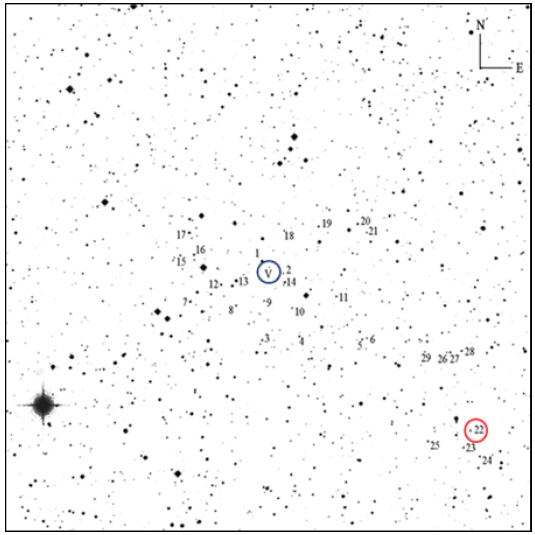
In total, we obtained 196 observations in V (range 16.51m–17.51m) and 242 observations in R (range 15.88m–16.77m) between 2012 and 2014. The total duration of observations was 45.5 hours during 11 nights in R and 8 nights in the alternatively changing filters VR. The time interval of the observations was JD 2455998–2456722. To improve calibration accuracy, we have used the method of “artificial comparison star” (Andronov & Baklanov 2004; Kim et al. 2004). As the object is in the field of V1323 Her, we have used the star C1 of Andronov et al. (2011), for which Henden (2005) published the magnitudes of V and R filters: V=14.807m, Rc=14.436m. The original observations (HJD, magnitude) are available upon request. Fig. 1 is the finding chart of V1323 Her with VSX1802.
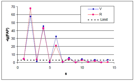
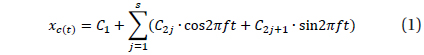
For the periodogram analysis, we have used the trigonometric polynomial fit of a degree s:

where coefficients

where

4. PHENOMENOLOGICAL MODELING. MULTI ? HARMONIC APPROXIMATION
The degree of the trigonometric polynomial
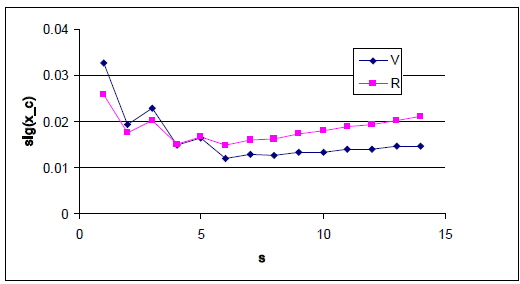
Another criterion proposed by Andronov (1994) is based on the r.m.s. estimate of the accuracy of the smoothing curve
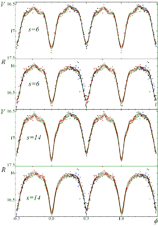
The phase curves in the V and R filters for statistically optimal degrees of trigonometric polynomial fit
5. PHENOMENOLOGICAL MODELING. THE NAV ALGORITHM
Phenomenological modeling of the light curves of eclipsing binary stars with relatively narrow eclipses was described in detail by Andronov (2012). The method was called “NAV” (”New Algol Variable”) and applied to a few Algol-type variables (e.g. Kim et al. 2010b).
In short, the method may be described as follows. The smoothing function is defined as usual in the linear least squares method

where

For

where phase is defined typically for a given initial epoch

A discussion of the computation of phase for the case of variable period may be found in Andronov & Chinarova (2013).
Another free parameter is the eclipse half-width
Other shapes used for determining of the parameters are based on a Gaussian function and its modifications (Mikulasek et al. 2012), which are formally of infinite width. An opposite approach is a splitting of the phase interval and approximation of the “out-of-eclipse” parts by a constant and of the eclipses by a parabola (Papageorgiou et al. 2014). The disadvantages of this model are: a) the discontinuity of the smoothing function, b) the underestimation of the depth of the minima because its width is set to a large constant and c) bad fitting of the ascending and descending branches. However, the number of parameters is only 5 (as the width of the eclipse and the phase shifts are set to constants).
Our previous approach was to use 5 parameters for the “constant+parabola” fit (brightness out of eclipse, at the primary and secondary minimum; half-width
In the NAV algorithm, the basic functions are:
f1(1)=1 f2(ϕ)=cos(φ), φ=2πϕ f3(ϕ)=cos(2φ) f4(ϕ)=sin(φ) f5(ϕ)=sin(2φ) f6(ϕ)=H((ϕ-ϕ0)/C8, C9) f7(ϕ)=H((ϕ-ϕ0-0.5)/C8, C10)
The coefficient
To continue numeration of the coefficients, we introduce
For each set of trial values of
Usually, the test function for one filter may be written in this way:

where
We have computed a dependence

The adopted value of the filter half-width

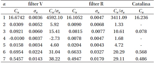
Coefficients of the phenomenological model for our observations in the filters V, R and that for Catalina (the latter published by Andronov et al. 2012).
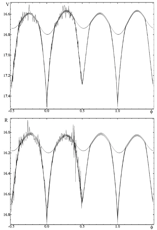
The corresponding light curves for the filters V and R are shown in Fig. 5.
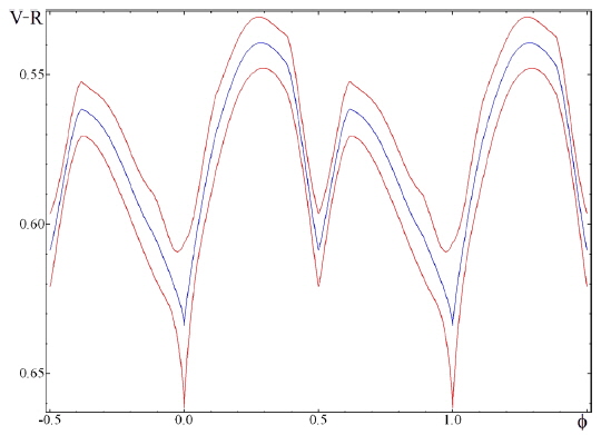
Using the smoothing functions for the two filters, the smoothing function of the color index V-R was computed. It is shown in Fig. 6.
From these coefficients of the “NAV” approximation, the classical phenomenological parameters listed in the GCVS (Samus et al. 2014) were determined: Max I=16.567m±0.006m, Max II =16.592m ±0.006m, Min I = 17.493m ± 0.014m, Min II =17.281m ±0.008m, Min I-Max I = 0.926m, Min IIMax I=0.714m (filter V). The corresponding point at the “depth – depth” diagram (Fig.1 in Malkov et al. 2007) lies close to the line “R” of equal radii, but slightly outside the allowed region. This is caused by the “simplified” model of spherical components without effects of ellipticity, reflection and limb darkening, which Malkov et al. (2007) have used.
The parameters
The mean color index, (V-R)=16.674m-16.105m =0.569m ± 0.069m was computed from the values of
These values of the color index are in the instrumental system, so, before taking into acco unt the color transformation coefficients and determining (V-R) in the standard system, we can't estimate more precisely the "color temperature" of the "star1+star2 system" (i.e. weighted mean temperature of two components) and corresponding "spectral class" (also intermediate between that of the components).
Following Andronov (2012), we introduce residual relative intensities


The intensities are in units of sum of intensities of two stars (out of eclipse, but "reduced" for the three effects mentioned above) and the “intensity depth” of minimum (how much light is eclipsed):
Andronov (2012) introduced a phenomenological parameter defined as

In the model of "spherical stars with no limb darkening" (Shulberg 1971; Malkov et al. 2005) recently discussed by Andronov & Tkachenko (2013b) as a "zero-order" approximation for determination of physical parameters), the eclipsed part of the light is proportional to the surface of projection at the eclipse
Let’s introduce
So one may write a system of 4 equations


with 5 unknowns,
However, we can estimate


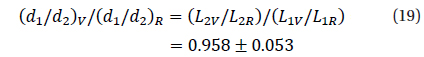
From this, we can derive another combination

i.e., equal to unity within error estimates. A small difference (even if smaller error), could be related to limb darkening.
Other combinations are for surface brightness


These phenomenological values may be used to estimate temperature ratios, e.g. using "Main Sequence" (MS) relations". From these MS assumptions, one may make a sequence of suggestions, which will be discussed below.
The second star (eclipsed at a primary minimum) has a larger surface brightness, consequently a larger radius and luminosity than the first star.
Taking into account Y≈1, one may suggest that the secondary eclipse is total (or close to total). Thus,


These values slightly differ by a value of 0.061±0.035=1.7

However, the (unknown) deviations from the mass-radius relation may exceed this maximal 5 percent difference in estimates using different coefficients of the statistical dependence.
From the duration of eclipse, one may suggest an inequality

For such large values, the stars are distorted (and we see this also from large values of
Although a possible W UMa – type classification may not be completely rejected, these stars are not yet in thermal contact (Lucy 1976) based on the difference of mean brightness and we suggest that they are not in contact. Thus, we perfer an EA - type classification with elliptic component(s).
Using the oversimplified form of the MS mass-radius relation

and, combining with Kepler's third law, we obtain the inclination,
Generally, these are minimal estimates of the radiuses and masses, since for an inclination,
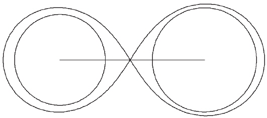
Even though the spectral classes of this system have not been reported yet, we can suggest the corresponding spectral classes of these stars to be G8 and K2 according to Cox (2000) and the possible Roche model of these VSX 1802 system can be estimated as in Fig. 7.
In this study, we estimated the paramaters only from phenomenological modeling of the phase light curve. The main unjustified suggestions were "no limb darkening" and "similar to MS dependencies" (no real quantitative relations, just "larger stars are brighter"). There are no detailed photometric or spectroscopic studies at present, therefore the true physical parameters of this system cannot be estimated for now.
Our phenomenological modeling could allow rough estimates to make the physical parameters. Although the errors of the phenomenological parameters are not very large (up to few percent), there may be systematic errors up to a dozen percent due to the simplicity of the model. These estimates may be used as preliminary values for further modeling using extended physical models based on the Wilson & Devinney (1971) code and it’s extensions (Wilson 1979, 1994, 2012, 2014; Zola et al. 1997, 2010; Bradstreet 2005; Kallrath et al, 2009; Linnel 2012; Reed 2012; Rucinski 2010; Prsa et al 2012). Such study of eclipsing binaries with the CBNU observations are reported by Jeong & Kim (2013); Kim & Jeong(2012); Jeong & Kim (2011) and Kim et al. (2010a). It should be noted that the lack of spectral data doesn’t allow to study various combination of stars in different evolutionary stages. Some discussions with crude assumptions about the age and metallicity of the system are therefore out of the scope of this study. More detailed photometrical and spectroscopic information will enable more thorough studies.


![Dependence of the r.m.s. value of the accuracy of the smoothing function σ[xc] on the degree of the trigonometric polynomial s.](http://oak.go.kr/repository/journal/16002/OJOOBS_2015_v32n2_127_f003.jpg)