The oceans are the largest global carbon reservoir, holding a total of about 38,000 gigatons of carbon, which is approximately 60 times greater than the total amount of carbon in the atmosphere and approximately 10 times greater than the total amount of carbon in the terrestrial biosphere and soils combined (Ciais et al. 2013). In addition, the fluxes of the Earth’s carbon reservoirs are associated with ocean processes, primarily in conjunction with their connection to terrestrial ecosystems. Among these oceanographic processes, organic carbon fixation by ocean primary producers and carbon exchange at the atmosphere-ocean interface comprise ca. 50% of the anthropogenic carbon (Sabine et al. 2004). Consequently, primary production in pelagic ecosystems accounts for a large percentage of global carbon sinks, and this topic is being actively studied in conjunction with the terrestrial ecosystems. In contrast, less attention has been given to carbon research in coastal ecosystems, likely because they occupy only a small amount (~7%) of the total ocean area (Borges et al. 2005). Furthermore, the input of allochthonous organic material from land and the high density of autotrophic organisms (e.g., vascular plants, macroalgae, phytoplankton, and microphytobenthos) add additional complications to coastal ecosystems, whereas only phytoplankton assemblages generally are considered in the open ocean. Consequently, it is more difficult to fully describe carbon cycles in coastal ecosystems, and more detailed descriptions of the processes important to these cycles are needed if we are to better understand them (Mcleod et al. 2011).
Carbon fixed by photosynthesis can follow several paths, one of which is burial beneath sediments. Although carbon a burial rates are high in coastal areas due to their high primary production, most coastal ecosystems that are dominated by autotrophic organisms (e.g., estuaries, mangroves, and salt marshes) generally act as net CO2 sources to the atmosphere due to overloading of allochthonous organic carbon (Chen and Borges 2009, Mcleod et al. 2011). Indeed, estuary and near-shore ecosystems show especially wide ranges of CO2 effluxes because of diverse sources of photosynthesis and respiration, anthropogenic inputs of carbon and nutrients, and heterogeneity of vegetative assemblages (Borges et al. 2005, Laruelle et al. 2010). In these systems, the high biomass of aquatic vegetation may play a crucial role in coastal carbon sequestration through the conversion of inorganic carbon to organic carbon during photosynthesis (Mcleod et al. 2011, Fourqurean et al. 2012). Consequently, these habitats are often referred to as “hot spots” because of their high carbon sequestration rates associated with rapid primary production. As a result, the global carbon burial budget in vegetated coastal ecosystems, which is estimated to be ~111 Tg C y-1, comprises about one-half of the total carbon buried in the oceans (Duarte et al. 2005) and represents a important portion of total ocean carbon sequestration. Therefore, understanding the rate of autotrophic carbon fixation is essential for better estimation of net carbon fluxes in coastal waters.
Among the oceanic processes that are significant factors connected with oceanic carbon flux, CO2 gas exchange is a relevant parameter associated with carbon flux in oceanic ecosystems in terms of net ecosystem exchange (NEE) (Lovett et al. 2006). NEE, which defines fixed and respired CO2 by individual organisms and populations, or even entire communities, is immensely important for understanding the coastal carbon cycle. Consequently, studies on coastal carbon cycles based on actual measurements of carbon flux parameters at the atmosphere-seawater interface are necessary to understand the roles of vegetation in the coastal carbon cycle.
Despite its importance, carbon mass balance in vegetated coastal ecosystems is difficult to interpret because constructing an adequate carbon model is a daunting job (Ver et al. 1999). In contrast, many conceptual models of carbon cycling have been developed for the open ocean (Randerson et al. 2002, Lovett et al. 2006). These models estimate coastal carbon cycles based on several biological and chemical parameters that are involved in the processes of converting inorganic and organic carbon. However, the organic carbon synthesized by photosynthesis in coastal areas can sink into the benthos, where it can be buried or transported away from the coastal ecosystem to offshore waters. Consequently, budgets of inorganic and organic carbon can be estimated by measuring the components associated with carbon sequestration, such as the net ecosystem production (NEP), the amount of allochthonous carbon input, the transport of carbon-rich material away from shore, and carbon burial rates at the benthos (Duarte et al. 2005).
Based on these perspectives, we focused on ecosystem production (NEP and gross ecosystem production [GEP]) and NEE in a highly productive coastal ecosystem to estimate carbon fluxes driven by autotrophic organisms. In this study, GEP, NEP, and NEE were quantitatively estimated in the Gwangyang Bay coastal ecosystem on the southern coast of Korea, where three communities of benthic autotrophs (eelgrass, macroalgae, and microphytobenthos) and a community of phytoplankton exist. Specifically, the objectives of this study were to 1) estimate GEP and NEP by photosynthetic carbon uptake and respiration of various autotrophs, 2) estimate NEE along the sub-ecosystem types (eelgrass beds, macroalgal beds, unvegetated shallow sediments, deep sediments, and deep rocky habitats), and 3) construct the conceptual box model of CO2 fluxes along the various vegetation types within the local vegetative coastal ecosystem.
>
Description of the study site
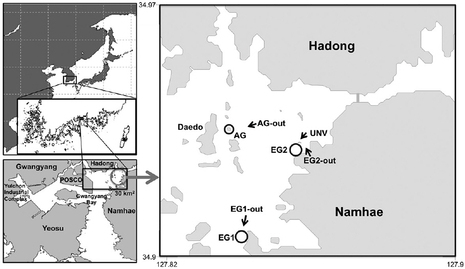
Gwangyang Bay is a shallow, semi-enclosed system, located on the south coast of the Korean Peninsula, whose hydrology is controlled by exchanges with offshore waters through a narrow strait (ca. 4 km wide) (Fig. 1). The maximum tidal range in the bay is approximately 4 m. The shallow coastal area (less than 10 m water depth) occupies more than 50% of the whole Gwangyang Bay area and is dominated by sediments comprised mostly of silt and clay. The primary source of allochthonous carbon and nutrients from land comes from the Sumjin River, although the Hadong coal-fired power plant and the Yulchon Industrial Complex located on the southwest corner of the bay are also potential sources of carbon, nutrients, and pollutants (Fig. 1). The autotrophic communities in Gwangyang Bay are comprised of phytoplankton, microphytobenthos, eelgrass (
In this study, the bay ecosystem was grouped into five habitats according to the dominant types of primary producers present and substrate characteristics. Specifically, these were 1) eelgrass beds (EG), 2) macroalgal stands (AG), 3) deep sedimentary habitats (UNV; >10 m), 4) shallow sedimentary habitats (EG-out; ≤10 m), and 5) deep rocky reefs (AG-out) (Fig. 1). The total area of each of these five habitats within a local box scale (30 km2 ) was estimated using a combination of image analysis of aerial photographs (Daum©, Samah©, Goyang, Korea) and shipboard surveys. These areas were 1) eelgrass beds = 1.9 km2 , 2) macroalgal stands = 1.6 km2 , 3) deep sedimentary habitats = 16.8 km2 , 4) shallow sedimentary habitats = 6.3 km2 , and 5) deep rocky reefs = 3.4 km2 . Following this, two eelgrass beds (EG1 and EG2) were selected to estimate primary production by eelgrass, phytoplankton, and microphytobenthos. One macroalgal stand (AG) was selected to determine the spatial distribution of each macroalgal species and phytoplankton and to estimate their individual rates of primary production. Four nonvegetated sites, two shallow sedimentary habitats (EG1-out and EG2-out), one deep sedimentary habitat (UNV), and one deep rocky reef (AG-out), were also selected, and primary production by the resident autotrophs was estimated. Finally, we developed a conceptual box model for carbon flux in the bay based on productivity estimates for the autotrophic organisms made between 20 June and 20 July 2007.
>
Daily radiation and environment factors
Down-welling irradiance was recorded continuously near the benthos at four of the sampling sites (EG1, EG2, AG, and UNV) using an LI-COR underwater photosynthetically active radiation (PAR) sensor (LI-192) connected to a data logger (LI-1400; LI-COR Inc., Lincoln, NE, USA) that was deployed during
Water temperature, salinity, and wind velocity were measured during seawater sampling, and these were used to estimate the pelagic productivity and CO2 gas exchange with the atmosphere. Specifically, temperature and salinity were measured using a HOBO Pendant temperature loggers (Onset Computer Corp., Bourne, MA, USA) and an 8410-A Portasal Portable salinometer (accuracy, ± 0.003; OSIL, Hampshire, UK), respectively. Data for wind velocity were obtained from meteorological observations collected about 14 km from the study sites.
>
Eelgrass and macroalgae biomass
Eelgrass shoot density was estimated within 13 to 15 quadrats (0.063-m2) that were haphazardly placed within each eelgrass bed by a SCUBA diver. The aboveground biomass of eelgrass for these samples was estimated using the average of the individual shoot weights within each quadrat, and the total area of the eelgrass beds within the bay was determined using a DT-X digital echosounder (Biosonics Inc., Seattle, WA, USA), with data collected using a high frequency transducer (420-kHz single-beam). The echosounder data showed that the eelgrass was distributed homogeneously among the study sites (Kim et al. 2008). Additionally, the biomass of macroalgal species was quantified by collecting all macroalgae within 0.063-m2 quadrats that were placed at 2-m intervals along a three transect line running perpendicular to the coastline at the AG site (n = 18 quadrats). After sample collection, the wet weight was measured to estimate individual species distributions, and the biomass of macroalgae within the samples was determined based on the sum of the different species. The total biomass of macroalgae in the bay was then estimated based on the total area of macroalgal stands and the mass and relative abundance of each species.
>
Productivity and respiration of eelgrass and macroalgae
To estimate rates of photosynthesis and respiration by individual eelgrass and macroalgae,
>
Productivity and respiration of pelagic phytoplankton
The pelagic primary production of phytoplankton at the eelgrass beds (EG1 and EG2) and at the deep rocky reef (AG-out) was determined by the 14C technique in order to estimate the phytoplankton contribution to ecosystem production. Seawater samples were filtered through a 200-µm mesh to remove large zooplankton and suspended particles. The resulting water and phytoplankton were then added to incubation bottles (ca. 80-mL cell culture flask; Corning), which were wrapped in layers of screen as was done with the macroalgae and eelgrass. Each bottle was inoculated with 10 µCi of NaH14CO3 and then incubated at
>
Productivity and respiration of benthic microbial mats
To estimate primary production and respiration by microphytobenthos in the soft sediments, sediment samples were collected from vegetated shallow sedimentary (EG2-in), unvegetated shallow sedimentary (EG2-out), and unvegetated deep sedimentary (UNV) regions. For this work, transparent acrylic tubes (ID 5 cm) were inserted ca. 12 cm deep into the sediment by a SCUBA diver without disturbing the surface sediments. Five intact sediment cores at each sampling sites were then moved quickly to the laboratory (within 5 h), where they were held under simulated field conditions of temperature, salinity, and light-dark cycle (23°C, S = 32, and 12 : 12 LD cycle, respectively). Additionally, the samples were acclimated to low light levels provided by daylight fluorescent lights (20 µmol photons m-2 s-1). Oxygen production by photosynthesis was measured with vertical oxygen microprofiles that were obtained using a Clark-type oxygen microelectrode (tip diameter 25 µm; OX-25; Unisense, Aarhus, Denmark), and net areal production and respiration of the microbial mat were calculated based on each oxygen microprofile after 20 min of exposure to seven different of light intensities, which were provided by a halogen illuminator (KL 2500 LCD; Schott, Mainz, Germany) (Kühl et al. 1996). The net community production (NCP) and respiration (
>
Net / gross community and ecosystem production
Photosynthetic parameters of eelgrass, macroalgal species, and microalgal communities (maximum photosynthetic rate, P
>
Determination of seawater pCO2 and NEE (CO2 exchange)
To determine the carbon chemistry in the seawater, surface seawater samples were collected from each site around midday. The samples were transferred quickly to 500-mL Pyrex bottles, without introducing air bubbles, and then immediately poisoned with 100 µL of saturated HgCl2 (Dickson et al. 2007). Concentrations of total dissolved inorganic carbon (
>
Daily radiation and environment factors
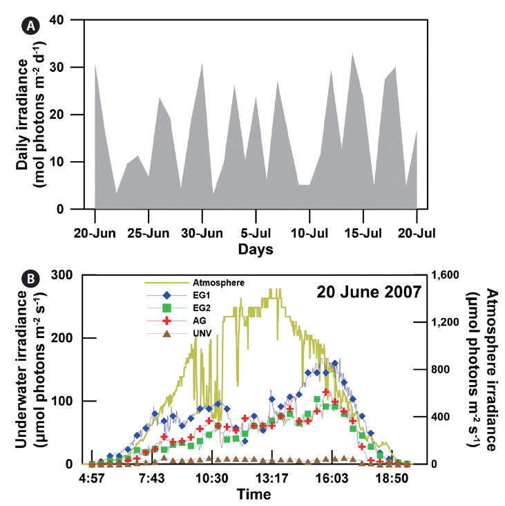
The daily atmospheric solar irradiance in the bay ranged from 3 to 33 mol photons m-2 d-1 during the study period (20 June to 20 July 2007) (Appendix 2A). Based on the estimated light attenuation coefficient, the surface irradiance was reduced to about 8-12% at the eelgrass canopy depth in EG1 and EG2 and to about 15-32% at the biomass-rich macroalgal site (AG). The irradiance at the shallow sediment (bottom of the eelgrass beds) was 5-8% of surface irradiance (Appendix 2B), and at the deep unvegetated sedimentary site (UNV), only 1% of surface irradiance reached the sediment surface. In contrast, water temperature and salinity were relatively consistent, ranging from 20 to 25°C and from S = 32.2 to 32.5, respectively. The mean wind velocity during the study period was 1.27 m s-1.
>
Eelgrass and macroalgal biomass
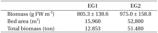
At eelgrass bed EG1, the aboveground eelgrass biomass was estimated to be 805.3 ± 138.6 g FW m-2. The area covered by the eelgrass and its total biomass was estimated to be ca. 15,960 m2 and 13 wet tons in June 2007, respectively (Table 1). At eelgrass bed EG2, the mean aboveground eelgrass biomass was estimated to be 975.0 ± 158.8 g FW m-2 and the area covered by the eelgrass and its total biomass was estimated to be ca. 52,800 m2 and 51 wet tons, respectively.
[Table 1.] Aboveground biomass, bed area, and total biomass at the two eelgrass beds in June 2007

Aboveground biomass, bed area, and total biomass at the two eelgrass beds in June 2007
At the macroalgal vegetation site (AG), eleven macroalgal species, of which two were green algae, three were brown algae, and six were red algae, were distributed along the subtidal rocky shore (Table 2). Among these, six species (
[Table 2.] Major macroalgal species and their mean biomass at the subtidal rocky shore in June 2007
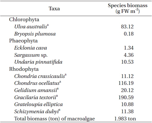
Major macroalgal species and their mean biomass at the subtidal rocky shore in June 2007
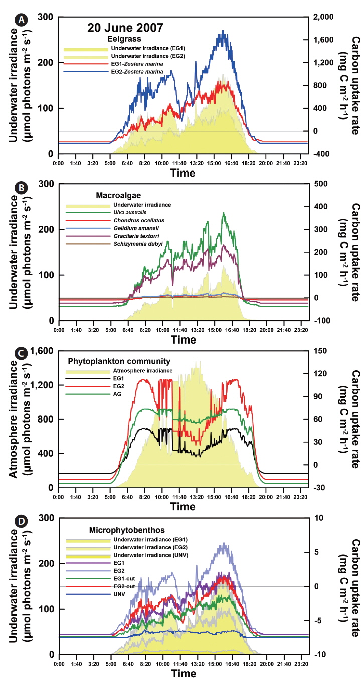
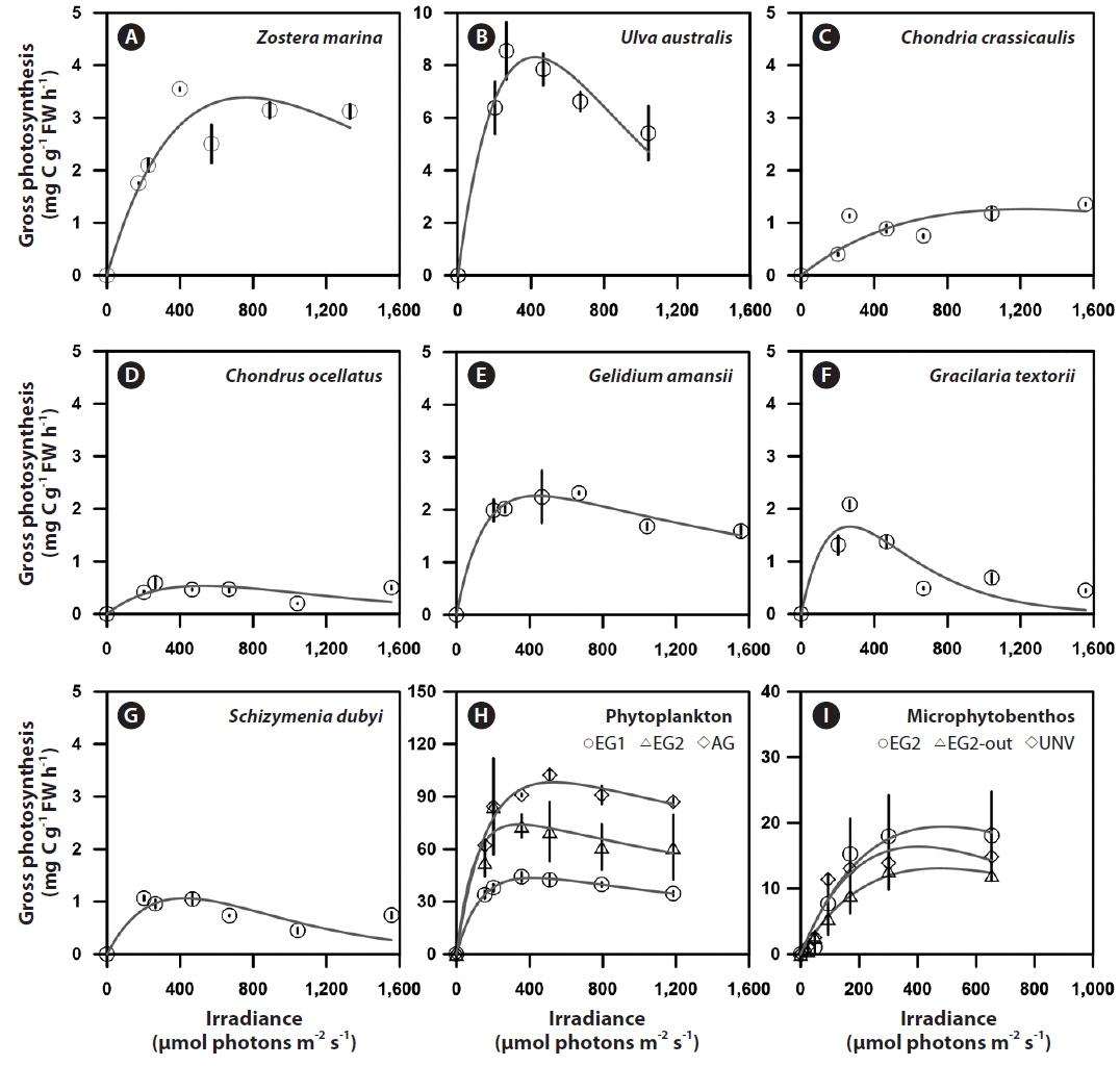
Photosynthesis varied among the eelgrass and macroalgal species, and its characteristics were clearly identified by photosynthetic parameters of the P-I curves (Appendix 3A-E). Specifically, the maximum photosynthetic rate (P
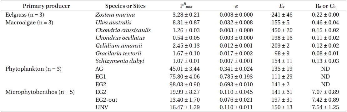
Photosynthetic parameters from each species or community calculated from P-I curve fits (Platt et al. 1980): the maximum photosynthetic rate (PB max), photosynthetic efficiency (α), saturating irradiance (Ek), and dark respiration (Rd) or community respiration (CR)
The photosynthetic characteristics of phytoplankton obviously differed by vegetation types, but those of the microbial community were not significantly identified with habitat types (Appendix 3H & I). Higher areal P
>
Community / ecosystem production and NEE
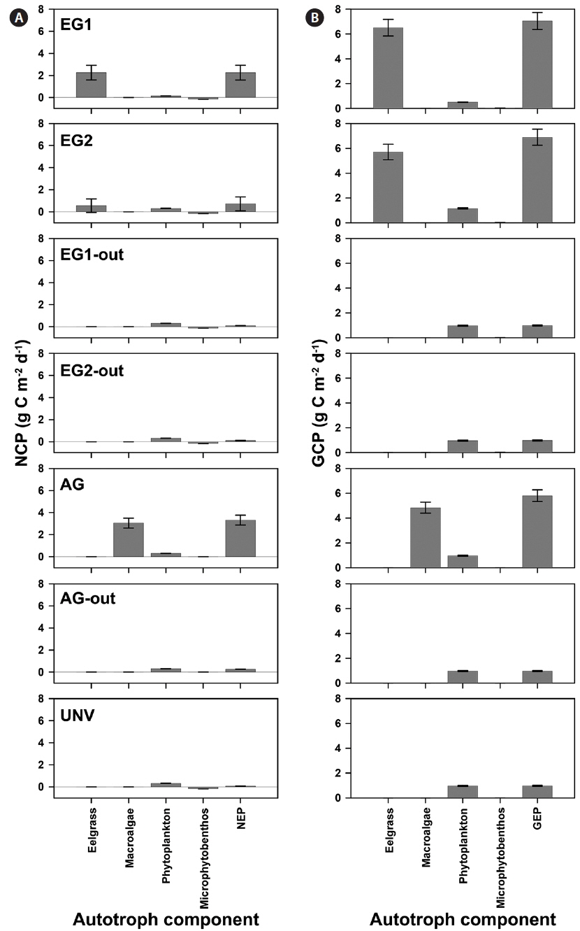
GCP was high in the vegetation communities, but a high rate of respiration is a potential countervailing factor for high GCP of the vegetation system. Specifically, the eelgrass and macroalgal communities exhibited extremely high NCP and GCP compared with those of the microalgal communities (phytoplankton and microphytobenthos) (Fig. 2). Additionally, the GCPs at the eelgrass beds were 6.51 ± 0.67 and 5.70 ± 0.62 g C m-2 d-1 in EG1 and EG2, and the NCPs of the eelgrass accounted for 35 and 10% of GCP at EG1 and EG2, respectively. The NCP at the macroalgal vegetation (AG) site accounted for 63% of GCP, and the GCP and NCP values were 4.83 and 3.05 g C m-2 d-1, respectively. The pelagic phytoplankton community was a net autotrophic system (mean value, 0.288 g C m-2 d-1), whereas the benthic microbial mat showed net heterotrophic communities (mean value, -0.156 g C m-2 d-1) irrespective of community type.
The high rates of GCP and NCP in the vegetation systems also led to higher values of NEP and GEP (Fig. 2). According to the NEP and P : R ratio (GEP to ecosystem respiration, Re), all study sites showed net autotrophic ecosystems, ranging from 0.09-3.31 g C m-2 d-1 for NEP and from 1.10-2.33 for P : R ratio (Table 4, Fig. 2). GEP was highest at the eelgrass habitat (EG1, 7.06 ± 0.68 g C m-2 d-1) due to the high productivity and biomass of eelgrass. Otherwise, the lowest GEP was observed at the unvegetated rocky shore (AG-out, 0.97 ± 0.04 g C m-2 d-1), where only phytoplankton production was considered. The highest NEP was found in AG (3.31 ± 0.45 g C m-2 d-1), along with the highest P : R ratio (2.33). Also, the eelgrass beds showed ca. 78% lower NEP (2.26 ± 0.67 and 0.73 ± 0.63 g C m-2 d-1 in EG1 and EG2, respectively) compared to GEP, even though these sites showed the highest GCP due to high ecosystem respiration.
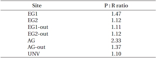
Monthly gross ecosystem production: ecosystem respiration (Re) ratio at each study site (20 June-20 July 2007)
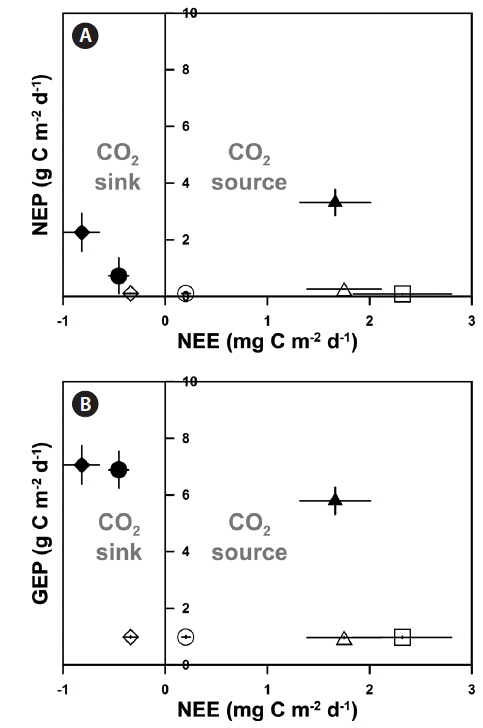
Based on the results of the seawater CO2 exchange measurements (NEE), the eelgrass beds (EG1 and EG2), which had high GEP with dense eelgrass, act as CO2 sinks (-0.81 ± 0.17 and -0.45 ± 0.09 mg C m-2 d-1 for EG1 and EG2, respectively). Additionally, EG1-out acts as a CO2 sink despite an NEP that was lower than those in the vegetation systems (-0.34 ± 0.07 mg C m-2 d-1). The other unvegetated sites (except for EG1-out) act as sources of CO2, for which the results ranged from 0.20 to 2.32 mg C m-2 d-1 (Fig. 3). Otherwise, AG acts as a CO2 source to the atmosphere even if this system is characterized by highly productive areas (1.66 ± 0.34 mg C m-2 d-1).
>
Conceptual model of the coastal carbon cycle
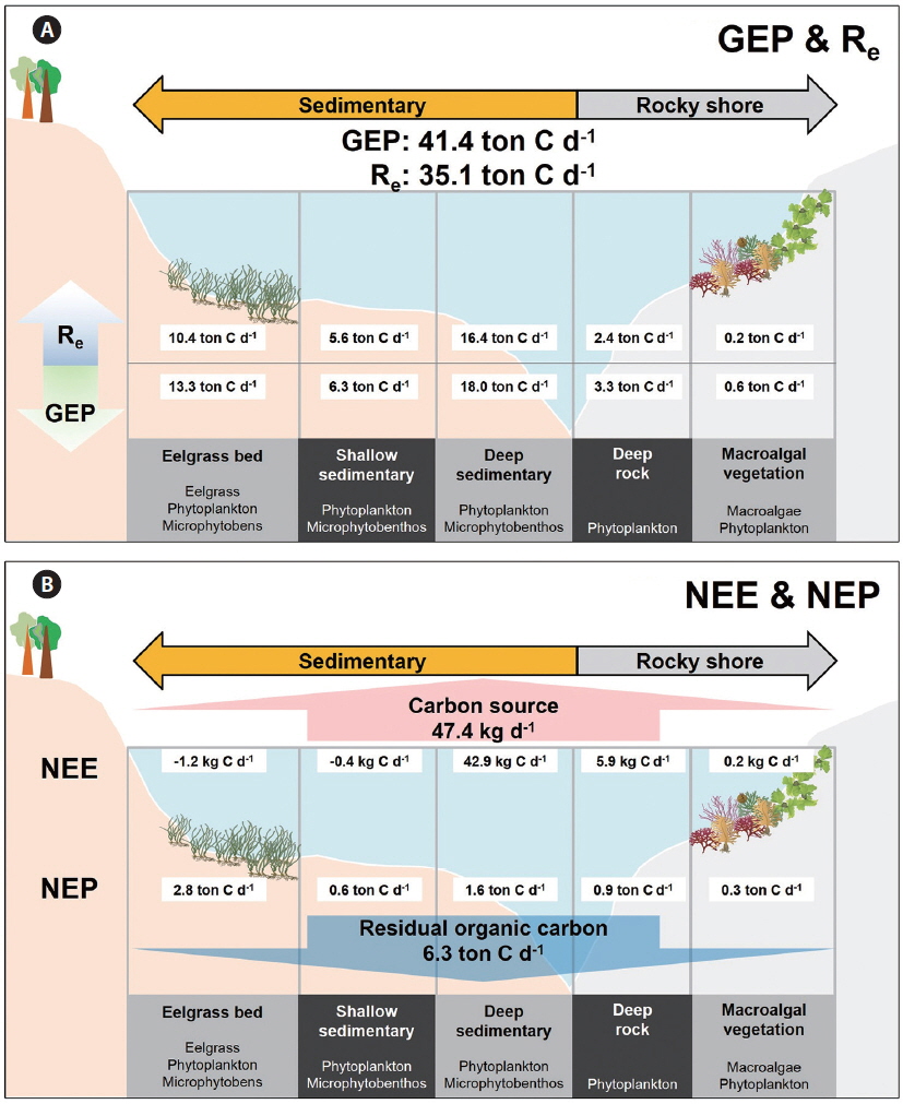
A conceptual diagram of the coastal carbon cycle, which puts ecosystem production and NEE along the various types of sub-ecosystems, is represented in Fig. 4 within a local box scale (ca. 30 km2 ). The entire Gwangyang Bay system uptakes a total 41.4 tons of inorganic carbon via GEP and releases 35.1 tons of CO2 through Re to coastal waters (Fig. 4A). Specifically, the deep sedimentary region showed the highest GEP of 18.0 ton C d-1. Although the eelgrass bed occupied only a small area, this system represents 73% of the bay’s GEP in the local box scale compared to the deep sedimentary habitats (13.3 ton C d-1). The macroalgal vegetation had the lowest GEP, NEP, and Re (0.6, 0.3, and 0.2 ton C d-1, respectively), presumably because the macroalgal habitat occupied the smallest proportion of the bay’s area. The eelgrass bed has the highest NEP among the sub-ecosystems (2.8 ton C d-1). Consequently, this embayment system has approximately 6 tons of carbon is potentially fixed as organic matter based on NEP, and some portion of photosynthesized organic carbon possibly sequestered to the outer sea. Also, approximately 47 kg of CO2 is emitted into the atmosphere from the seawater, as estimated by NEE.
Although many studies have attempted to describe coastal carbon cycles, there have been limits to quantify carbon budgets within vegetative coastal ecosystems, and additional efforts are still required (Tokoro et al. 2014). For example, some studies have focused on biological metabolism and carbon mass balance approaches within ecosystem production based on gas exchange and NCP (Bates et al. 1998, Sarma 2003). Additionally, carbon flux has been estimated by comparing net ecosystem production to gas exchange in an estuary system (Pradeep Ram et al. 2003). However, these studies have been largely restricted to unvegetated areas where only phytoplankton and / or microphytobenthos were considered. Otherwise, some studies have focused on biological metabolism to estimate the carbon balance in vegetative coastal habitats. The carbon budgets in vegetation-dominated habitats have thus been estimated by measuring primary production. However, these studies have not considered many of the complicated carbonic parameters, such as gas exchanges with the atmosphere (Frankignoulle and Bouquegneau 1987, Kaldy et al. 2002). To address these deficiencies, our investigation was conducted to establish a conceptual box model for coastal carbon fluxes, with attention to carbon mass balance based on ecosystem production and CO2 gas exchange in various types of vegetated and unvegetated systems.
Coastal vegetated ecosystems are generally characterized as highly productive areas, and our production / respiration data support this. All of the sub-ecosystems in our study were autotrophic in nature (i.e., P : R ratio >1) (Table 4), with production : respiration ratios comparable to those found in other studies (e.g., seagrass bed, 1.19- 1.50; unvegetated habitats, 0.03-34.3) (Duarte and Agusti 1998, Ziegler and Benner 1998). Although Gwangyang Bay was a sufficiently productive environment during the experimental period, as shown by the P : R ratio, not every sub-ecosystem acted as a CO2 sink from the atmosphere. This is not surprising given that many coastal ecosystems with vigorous biogeochemical activities can act as CO2 sources to the atmosphere (Borges et al. 2005). Our NEE results showed that a heavily vegetated bay could act as both a sink and source of CO2 depending on the type of vegetation present (Fig. 3). Specifically, our two eelgrass beds acted as CO2 sinks, presumably because of the high photosynthetic activity of the eelgrass and the near-stagnant seawater. These environmental traits may lead to a reduction of
The NEP (integration of pelagic and benthic NCPs) in the coastal ecosystem is a key factor associated with carbon export to the region outside of the coastal system (Duarte et al. 2005), and it is particularly important in the aspect of carbon sequestration because a significant portion of the exported carbon can be moved to the open ocean or become buried in sediment. Especially, submerged aquatic vegetation showed significantly high ecosystem production (Kaldy et al. 2002). Thus, the production of benthic autotrophs is an important component of the coastal ecosystem with respect to regulating the carbon cycle, and it could enhance the organic carbon sequestering efficiency (Mcleod et al. 2011). The areal NEPs partitioned by the five types of coastal sub-ecosystems (eelgrass bed, macroalgal vegetation, shallow sedimentary, deep sedimentary, and deep rocky) were substituted to construct the conceptual diagram of carbon flux in the local coastal system (see Fig. 4). The estimated NEP value in the local box scale (30 km2 ; northeastern part of Gwangyang Bay) was about 6.3 ton C d-1, which could be expressed as the organic carbon mass balance (Fig. 4A). Especially, the NEP in vegetated habitats (eelgrass and macroalgal beds) exhibited 33% of GEP in a whole are of studied site (30 km2 ), even though these habitats occupied only 12% of the total area. If vegetated coastal ecosystems produce an overload of photosynthesized organic carbon, it may lead to an increase in the rate of carbon sequestration (Barrón et al. 2003). There are two important pathways for understanding the fate of fixed organic carbon in the coastal ocean (Ver et al. 1999). A portion of the exported carbon will be either 1) transported to the open ocean (dissolved and / or particulate organic carbon) or 2) buried in the sediment. The organic detritus on the upper layer of the sediments could af-fect the oxidation and recycling of nutrients (Giusti and Marsili-Libelli 2005) and be exported to the marginal sea through the “continental shelf pump mechanism” (Tsunogai et al. 1999). However, quantification of the organic carbon cycle in the vegetated coastal ecosystem via these two pathways was not addressed by our research, thus these factors remain as topics for future research to clarify the coastal organic carbon cycle. Another minor possible pathway of exported carbon is that it is 3) emitted to the atmosphere. Our NEE results quantified the CO2 emitted to the atmosphere and showed that our local coastal area emits approximately 47.4 kg d-1 CO2 into the atmosphere, which is about 200 times smaller than NEP. This level is small compared to ecosystem production, but CO2 gas exchanges at the atmosphere-seawater interface have yet to be explored in relation to the ecosystem production of various vegetation systems.
This study would be remarkable indeed, since many measurable parameters were considered in relation to coastal carbon flux such as biomass, productivity of various coastal autotrophs, and CO2 exchanges with
In summary, this study provides an example of how to use a mass balance approach to integrate estimates of carbon flux with measurements of photosynthesis and CO2 gas exchange in a complicated coastal vegetated system. Based on our results, we quantified carbon flux over the short-term in a bay ecosystem using the model proposed. Although, our conceptual box model does not consider all the complicated biological activities and environmental fluctuations, it is sufficient for evaluating short-term and local-scale estimations of carbon flux. Additionally, we presented a conceptual box model that can be applied to other vegetated systems in order to estimate coastal carbon cycling. To achieve this aim, additional parameters about carbon chemistry in seawater need to be considered. These include the fate of dissolved inorganic carbon, particulate / dissolved organic carbon, and hydrological parameters and carbon mineralization for the long-term and large-space scale.