LIDAR (LIght Detection And Ranging) is a well-established technique not only for atmospheric remote sensing and terrestrial hydrography, but also for coastal bathymetry and topography [1-3]. In contrast to the wide possible applications, LIDARs are mostly implemented in atmospheric environments in Korea. Only recently great efforts have been paid to developing a laser bathymetry system based on a pulsed green laser with an emphasis on underwater object detection [4].

Numerical techniques for the radiative transfer of an under-water light field have been extensively investigated because understanding the propagation character of a light field in coastal water is a fundamental issue in LIDAR bathymetry as well as in other fields [5]. Various models for computing underwater light distributions have been in use, e.g. the discrete-ordinate-method [6], the invariant imbedding method [7], and the Monte Carlo method [8]. In particular, the Monte Carlo (MC) method has served as a useful tool to model the distribution of underwater downwelling irradiance in the coupled atmosphere-ocean system, the reflected solar background from the water surface, and the waveform analysis in the time-resolved form [9]. In most cases, however, the MC simulation has been used for common ocean optics applications, e.g. the modeling of natural ocean-atmosphere environments under a point source like sunlight.

In this paper, we present the radiative transfer of a conventional laser beam, e.g. a Gaussian beam, in a water medium using the Monte Carlo method. The redistribution of a fraction of the photon energy in the original Gaussian beam and in the scattered beam during propagation is described. The dependence of the beam propagation behavior not only on the inherent optical property of the ocean water like the single scattering albedo, but also on the laser beam parameter, e.g. the M squared factor is discussed. In addition, several design considerations for a bathymetric LIDAR are discussed.

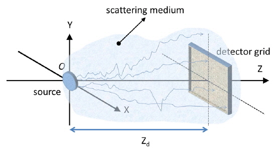
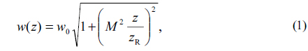
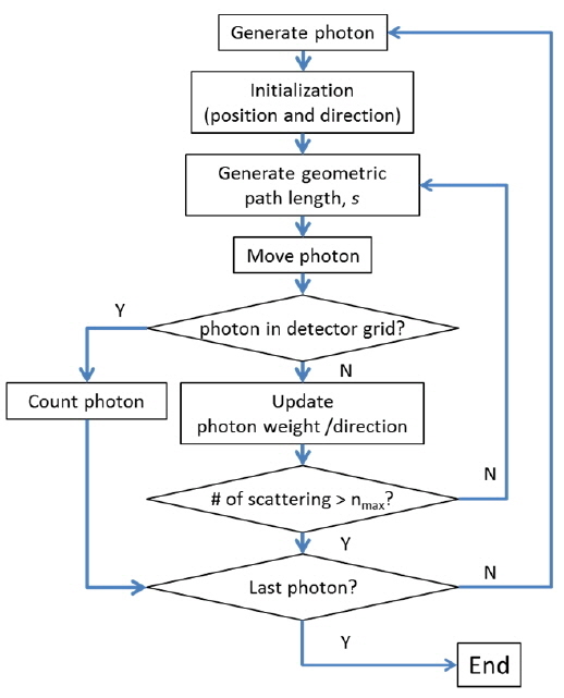
Figure 1 shows the geometrical schematic of the simulation. Photons in a Gaussian distribution start to travel at (x, y, 0). In a scattering medium with a total attenuation coefficient, c (c = a + b, where a is the absorption coefficient and b is the scattering coefficient), photons are absorbed and scattered as they propagate. At z = z_d, an arrayed detector is placed to count photons which arrive at the detector grid. The logical flow for calculation is well described in the flow chart in Fig. 2. The Mathematica 10.0 program is used for the coding. The spot size of a Gaussian beam at a distance, z, is determined by the conventional Gaussian beam theory [10]:

where w₀ is the 1/e² spot size of the laser beam, z_R is the Rayleigh length (=πw₀² /λ), and M² is the beam quality factor. The radial position of a photon in a Gaussian distribution is sampled by [11]:

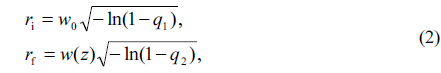
where r_i and r_f are the initial and final radial position, respectively, q_i is a random number ranging from 0 to 1. The initial direction cosine is determined by the angle between the r_i and r_f. For validation, the free space propagation of a Gaussian beam is simulated by MC algorithm and compared to the conventional, showing good agreement.

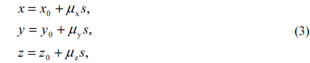
Once the initial position as well as the direction is determined, a photon travels a geometric path-length, s (=ln(q)/c), and the position of the photon is updated by:

where (x₀, y₀, z₀) is the previous coordinate, (μ_x, μ_y, μ_z) is the direction cosine. After a scattering event, the direction cosine should be appropriately updated. For validation of the direction update, the diffusion of a point source in an isotropically scattering medium is simulated yielding a good agreement with the diffusion theory. The scattering character in this study is determined by the Henyey-Greenstein phase function [12]:

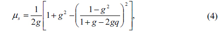
where g is the asymmetry factor. For coastal water, the asymmetry factor is taken to be 0.9 [13]. In each scattering event, the photon weight should also be renewed by:

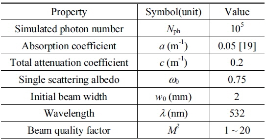
where ω₀ =(c−a)/c is the single scattering albedo. The parameters in use for the simulation are listed in Table 1.

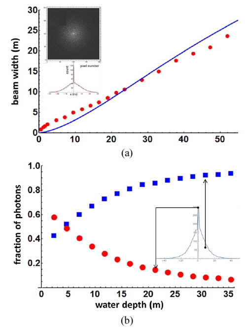
The inset of the Fig. 3(a) shows a density plot of the laser beam and its projected profile at z = 1.1 z_R (~ 26 m). There is a strong peak in the center, which is from the original Gaussian beam, while the scattered photons are distributed around the center peak. As the laser beam propagates in a water medium, the photons are scattered and the width of the scattered photon distribution is widened as shown in Fig. 3(a). The 1/e² width of the scattered photon distribution (red dots) is deduced by a Gaussian fitting of the projected beam profile. For the given condition in the Table 1, the width grows as large as 10.8 m at z = z_R (~ 23.6 m), which far exceeds the original beam width. The widths deduced by the MC method are compared with the results of Lutomirski’s theory (blue line) [14, 15], yielding good agreement. For calculation by the analytic model, the wave-slope variation (σ_x,y), rms scattering angle owing to maritime aerosols (σ_β) are neglected and the incidence angle is set to 0, and the root-mean-square scattering angle (Θ_R) is calculated by the asymmetry factor g. The diffuse attenuation coefficient (K_d) is deduced by inherent optical properties in Table 1 [16]. Figure 3(b) shows the variation of the fraction of photons in the center peak (red dots) and in the scattered distribution (blue rectangles) at various depths. As the laser beam propagates, the fraction of photons in the center peak decreases, while the energy in the scattered distribution increases. This can be understood in terms of the redistribution of the energy in the center peak into that in the scattered distribution through the diffusion. After the beam reaches a depth of z = 1.6 z_R (~ 38 m), the center peak completely disappears, thus only the fraction of the photons in the scattered distribution propagates. The conventional amplitude of the return signal from a target, e.g. sea bed and an underwater object is mainly contributed by the original Gaussian photon fraction because the scattered photons are scattered out. Thus the maximum detectable depth using a LIDAR return signal can be expected to be more or less 38 m in the given environmental condition. On the other hand, the maximum detectable depth can be further extended by increasing the output energy of the laser and detecting tiny a fraction of the photons in the scattered distribution using a single-photon detector, e.g. a photomultiplier tube. In this case, the field-of-view loss factor induced by the broad distribution of scattered photons should be appropriately estimated for the optimized LIDAR performance [15, 17].

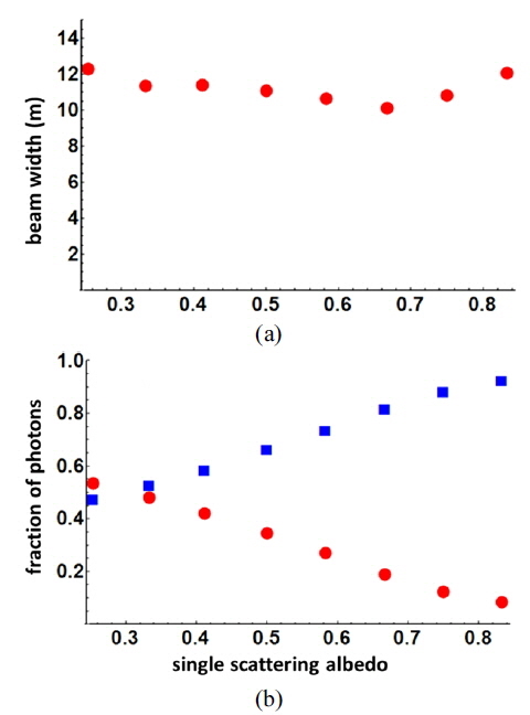
The width of the fraction of the photons in the scattered distribution as a function of the single scattering albedo (ω₀) at z = z_R is shown in Fig. 4(a). For the calculation, the water absorption is fixed to be 0.05/m. The influence of the single scattering albedo on the beam width of the scattered fraction is not critical. The standard deviation of the various beam widths is only 6.5 % of the mean width. Thus, the environmental parameter is not the major factor in the beam spread of the laser beam in the scattering medium. Figure 4(b) shows the energy redistribution behavior as a function of the single scattering albedo. The fraction of photons in the original Gaussian beam (red dot) starts to significantly decrease at ω₀ ~ 0.33, while the fraction of photons in the scattered distribution (blue rectangles) starts to increase at this point. It can be easily expected that the return signal amplitude starts to be degraded at ω₀ ~ 0.33 in the given laser output energy.

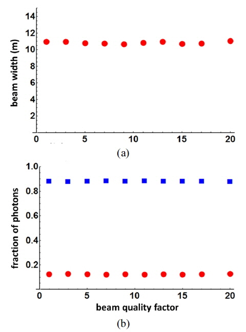
In Fig. 5(a), the dependence of the scattered beam width on the beam quality factor for z = z_R is shown. For various beam quality factors ranging from the ideal case (1.0) to the multimode case (20.0), the scattered beam width is almost constant at ~ 10.9 m. Furthermore, the fraction of photons, i.e. the averaged energy density has no influence on the beam quality factor as shown in Fig. 5(b). The photon fraction in the Gaussian beam and the scattered distribution are almost constant at 0.13 and 0.87, respectively. This result shows that the propagation behavior in terms of the averaged energy density in the original Gaussian beam and the scattered photon distribution is independent of the M-squared. This is true even if the fine structure of the Gaussian beam is distorted when taking refractive index fluctuations of the coastal water as well as the random evolution of the ocean surface into account. These factors are not considered in the current calculation [13, 17]. Thus any laser source with high beam quality is not required because the initial beam quality diminishes during the propagation after a distance, e.g. longer than 38 m in the given environmental condition. In a practical point of view, the effort required to maintain single mode character in high power laser for a bathymetric LIDAR system can be significantly reduced.

In conclusion, the Monte Carlo simulation for underwater propagation of a Gaussian beam was performed and the results were presented. The variation of a fraction of the photon energy in the original Gaussian beam and in the scattered beam during propagation was simulated. The dependence of the beam propagation behavior on the inherent optical properties of the ocean water like the single scattering albedo and on the laser beam parameters, e.g. M² factor was discussed. The results may offer several design considerations of a bathymetric LIDAR, e.g. the field-of-view loss factor, the requirement of single mode character of the laser.

The simulation can be further improved by including the random ocean surface, the measured volume scattering function, and the measured IOPs, e.g. the absorption coefficient, the single scattering albedo.