Active optics is a key technology for future large-aperture space telescopes. In the design of deformable mirrors for space applications, the design parameter trade-off between the number of regularly configured actuators and the correction capability is essential but rarely analyzed, due to the lack of design legacy. This paper presents a parametric module method for integrated modeling of deformable mirrors with regularly configured actuators. A full design parameter space is explored to evaluate the correction capability and the mass of deformable mirrors, using an autoconstructed finite-element parametric modeling method that utilizes manual finite-element meshing for complex structures. These results are used to provide design guidelines for deformable mirrors. The integrated modeling method presented here can be used for future applied optics projects.
With the increasing demand for earth observations and astronomy surveys, space telescopes have been driven to evolve towards designs with large apertures, wide fields of view, and agile observation. However, the optomechanical design of large-aperture space telescopes is still one of the most challenging tasks in space projects.
The difference in gravity between fabrication on Earth and operation in space leads to a constant bias in optical structure. Image quality degradation occurs due to the change in optical structure and the figure error of optical surfaces, which are caused by gravitational effects, thermoelastic distortion, and structural vibration. A rational optomechanical design of a space telescope is required to maintain stability of the optical structure under environmental disturbance. Meanwhile, both weight and size restrictions should be met for space applications; therefore, a lightweight design is essential for large-aperture space telescopes [1].
For small-aperture optics, high system stiffness can be obtained by using a lightweight structure and a material with high Young’s modulus [2]. Image quality degradation due to the changes in environment will be acceptably controlled by a proper design and tolerance budget.
Unlike small-aperture optics, system weight and size will count against the lightweight design if large-aperture optics also pursue a high-system-stiffness design to guarantee optical structure stability. The constraints of launch weight and size are violated, which makes the system unachievable. On the other hand, the fact that large-aperture optics are more sensitive to gravitational effects and thermoelastic and structural vibrations makes it even harder to design for space applications [3-5].
Therefore, to achieve a very lightweight design with excellent performance, large-aperture optics must use active methods, namely active optics, to correct optomechanical constant bias, misalignment, and system wavefront error caused by environmental issues. Active-optics technology has only recently been applied to space telescopes. For example, the James Webb Space Telescope (JWST), which is planned to be launched in 2018, will be implemented with multiple active-optics sets. With an active primary mirror whose diameter is 6.5 m (F/1.2), the JWST reaches the diffraction limit at a wavelength of 2 μm [6].
Space active optics mainly has the following two solutions in application.
One approach uses an active primary mirror, such as in the Hubble Space Telescope (HST) and the JWST mentioned above. The HST’s primary mirror has 24 actuators to compensate for lower-order aberrations, while the JWST’s primary mirror consists of 18 mirror segments, each with 7 degrees of freedom to compensate for rigid body movements and curvature change. The current state-of-the-art active primary mirror is the actuated hybrid mirror (AHM) developed by the Jet Propulsion Laboratory (JPL) [7], with a fast fabrication process, low areal density, and wavefront-correction capability making it promising for an extreme large-aperture space telescope [8].
The other approach uses exit-pupil deformable mirrors (DMs). Given that the aperture stop is on the primary mirror [9], which is more sensitive than other optical elements to environmental loads due to its size, a real exit pupil is required where a small, deformable mirror is placed to be conjugate to the primary mirror and to compensate for its figure error and the system wavefront error. This kind of DM is studied in this paper.
Unlike adaptive optics applied in large ground-based observatories, space active optics is dedicated to compensating for lower-order and larger-amplitude optical aberrations, and works at much lower frequency [10]. Existing DMs cannot be directly used in space applications because of operation specifications and critical restrictions for reliability and weight, size, power consumption, etc. For space applications, multidisciplinary constraints should be addressed, and a lot of effort is needed to make a technological breakthrough for DMs in future large-aperture space telescopes.
In general, the more actuators a deformable mirror has, the more degrees of freedom, and the better correction capability it can achieve. Due to the absence of design heritage, the design parameter trade-off that is essential to the design of DMs is still unexplored, and the optimal design of a DM is unknown, up to now.
S. K. Ravensbergen [11] developed a semianalytical model (ignoring edge effects) to describe thin facesheets on discrete actuators, using the plate theory of elasticity. However, this model is limited in providing a starting point, as its data is not suitable for further analysis. An analytic approach for DM design is difficult due to the lack of proper theory.
A parametric modeling tool [12] has been developed by the Space Systems Laboratory (SSL) at MIT to assist in the preliminary design of next-generation, lightweight space telescopes. The automatic-construction method in that tool for modeling an active-segment mirror is a valuable approach for parametric modeling [13], although the method is only available for simple structures and when low-fidelity finite elements are used.
NASA’s new mirror-modeling software [14] can automatically generate both mirror and suspension-system elements in several minutes, which makes the integration of these models into large telescope or satellite models easy. However, this software can only deal with a predetermined substrate pattern, and a relatively simple structure model.
Due to the lack of fully developed automeshing technology [15], high-fidelity finite-element models (FEM) are still built by manual meshing, which is time-consuming and impractical for large-volume design of experiments (DOE). The existing auto-construction method is quite limited to simple and regular structures [16], using low-fidelity elements for many parts (
To provide design guidelines for DMs, a new parametric module method for integrated modeling of a DM with regularly configured actuators is presented, by using an auto-construct parametric finite-element modeling method that takes advantage of manual finite-element meshing for complex structures. The method is practical for other applications as well.
The paper is organized as follows: Section 2 presents the large-aperture space telescope and the parametric module method. Section 3 describes the details of application of the parametric module method to the DM parametric modeling. Section 4 describes the integrated modeling process of DM figure compensation and the metric of correction capability. Section 5 presents the design trade-off carried out on a DM 320 mm in diameter, and Section 6 concludes the paper.
II. LARGE-APERTURE SPACE TELESCOPE AND PARAMETRIC MODULE METHOD
2.1. Large-Aperture Space Telescope Description
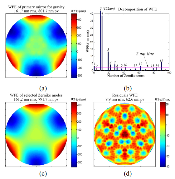
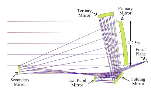
The large-aperture space telescope employs a 5-mirror telescope design with three off-axis mirror anastigmatic (TMA) optics and a focal length of 20 m, F/10, as shown in Fig. 1. The primary mirror is a monolithic light-weighted mirror of Φ = 2.5 m, conjugated with an exit-pupil mirror 320 mm in diameter. Although the primary mirror is made of silicon carbide (SiC), which has a very high stiffness-to-density ratio, the primary mirror is deformed dramatically under gravity due to its size. The wavefront error (WFE) of the primary mirror for 1
[TABLE 1.] Main components of the WFE of the primary mirror for gravity
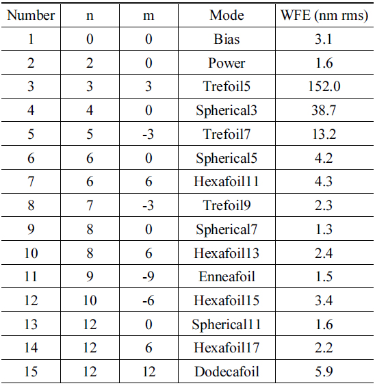
Main components of the WFE of the primary mirror for gravity
2.2. DM Design and Parametric Module Method
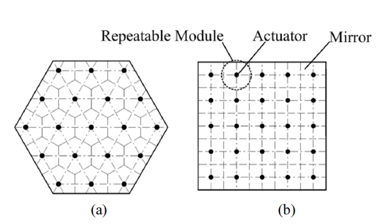
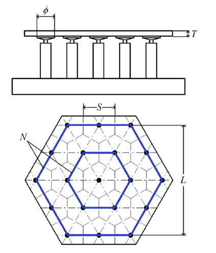
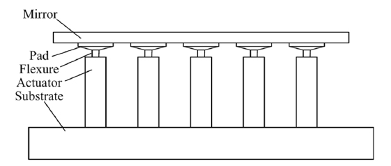
The structure of a continuous facesheet DM with discrete surface-normal actuators is described in Fig. 3. The desired figure on the mirror is generated by commanding actuators to work in a specified manner. Inner stress and the actuator print-through effect are relieved by using the Pad and Flexure. Generally, because of fabrication concerns, actuators of a DM are configured in a regular pattern; see Fig. 4. Moreover, note the dashed lines across the mirror; it is clear that the mirror can be divided into similar parts.
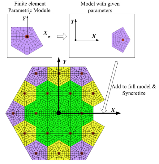
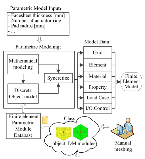
Figure 5 shows the approach to Parametric Module Modeling. Based on the fact that a DM with complex structure can be divided into repeatable parts, similar parts are defined by a module that is modeled by manual meshing and parametrized into a Parametric Module by using the object-oriented programming method. DM modules with similar Properties and Methods are defined by a Class, which is easily organized and operated.
Properties of the DM Class designed for the DM modules consist of the Parameter that presents the dimensions of the module, the FEM information including FEM data for the module (
Methods,
Managing the complexity of large modeling applications is improved by applying an object-oriented approach. By using parametric module modeling, discrete parts of the DM are generated from the DM modules defined by the DM Class and operated to possess a calculated position, orientation, and dimensions. The FEM of the DM is constructed by syncretizing the FEM of all parts. According to the solver deck used in finite-element analysis, the FEM of the DM is written into an FEM input file in a specified format, and finite-element analysis is then conducted.
The parametric method is useful for integrated modeling of complex structured models by combining manual finite-element meshing with the autoconstructed meshing method. The parametric and automated nature of this method allows large-volume design iteration.
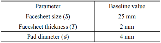
The parameters of the DM used in this paper are illustrated in Fig. 6. They consist of the effective aperture size
[TABLE 2.] Baseline for DM parameters
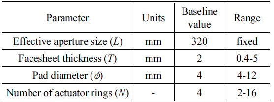
Baseline for DM parameters
The DM Class is designed according to the character of the DM module. Details of the DM Class and the whole model-building procedure are explained as follows.
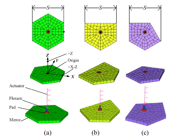
Figure 7 shows the FEM of several DM modules. It is clear that these modules have common structural features and parameters; thus, the properties of the DM Class are defined.
The independent dimensions of the DM module are stored in the Property Parameter, which includes the Character size
[TABLE 3.] Baseline for DM module parameters
Baseline for DM module parameters

The Property FEM Info reserves information describing the FEM (
The Property Accessory contains the Local coordinate of the DM, the Interface of the FEM, and the Node/Element Sets to be used in operations by declaring parts of the DM module. The local coordinate is determined by three points: the origin point of the local coordinate, a point on the +Z axis, and a point on the +X-Z plane. The local coordinate does not need to be the same as the global coordinate in which the FEM is defined. It is useful for ensuring that all parts of the DM model are consistent. Node/Element Sets are used for grouping parts of the FEM as components to make FEM operations possible.
Driven by the application of the DM module, several Methods are designed to update the FEM Info of the DM module according to the associated parameters. The Methods used in this paper include:
The rigid transformation of FEM The mirror operation of FEM The parameter update of FEM
The Methods change the nodal coordinates of the DM module by transforming or scaling the associated Node/Element Sets that are stored in the property of the DM module. Note that the method of scaling the FEM is limited according to the element uniformity of the DM FEM. To obtain high fidelity in analysis, a set of DM module pairs with different mesh densities are needed in application. Moreover, the Methods defined in the DM Class can be extended for future applications.
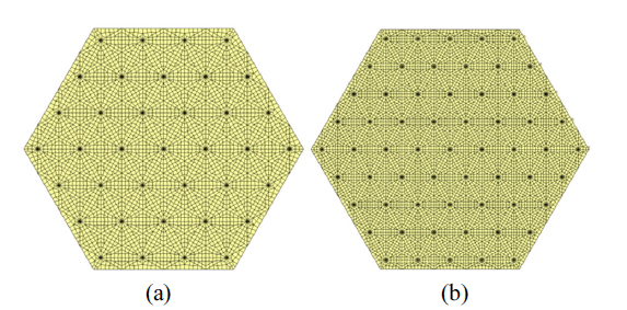
Once the DM modules have been built according to the definition of the DM Class, the DM model can be constructed by assembling all parts of the DM that are computed from corresponding DM modules. See Fig. 8. For example, one part of the DM model is updated from the DM module by modifying its dimensions, location and orientation predefined for the whole model. Then, through synthesis, this part is added to the whole DM model. According to the solver deck being used, the whole DM model and associated boundary conditions are written into an FEM input file in the specified format. Given the desired parameters, it takes mere minutes to construct the DM model. Figure 9 shows two DM models made up of different numbers
IV. DM CORRECTION CAPABILITY ANALYSIS
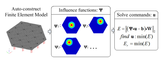
Shape control based on influence function has been chosen as the standard. It is divided into two types: the Zernike influence function and the Nodal influence function. It is convenient to acquire the Nodal influence function by extracting the surface nodes’ displacements from the results of finite-element analysis in which each actuator is given a unit command. The Zernike influence function has a spatial bandwidth limitation, and any portion of the shape disturbance that lies above the bandwidth of a set of Zernike polynomials is missed, so the residual error of Zernike fitting for the shape disturbance may be large and unacceptable[17]. The Nodal influence function is preferred in this paper, since computational cost is not a concern in this research.
The integrated modeling approach to DM correction capability analysis is illustrated in Fig. 10. Based on the parametric module method modeling described above, after a “unite” input is given to each actuator, the influence functions are obtained, and then the commands of object figures and the correction capability criterion are calculated.
Consider

The WFE of the primary mirror due to gravity is chosen as the object figure to estimate the DM cDM correction capability. The residual WFE should be controlled to within λ/50 rms. Object figure b ∈ ℜ
It is assumed that the DM is a linear system when deflections are much smaller than the size of the DM, and the surface figure of the DM under actuation can be obtained by superimposing surface figures under the motions of associated actuators. Meanwhile, the surface nodes of the DM FEM are distributed nonuniformly, so a weighting matrix W is used to address the area weight for each node. Hence, the control vector u containing commands for associated actuators, can be computed via the influence matrix by minimizing the RMS of residual deflection of a figure,


V. DM DESIGN TRADE SPACE ANALYSIS
There are 4 design parameters (L,
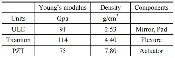
[TABLE 4.] Materials properties used in DM design

Materials properties used in DM design
A full trade space of designs is enabled by integrated modeling. There are three design parameters and two independent metrics (correction capability and mass). Via full-level design of experiments (DOE), all possible design cases can be evaluated.
5.1. Design Trade Space Analysis
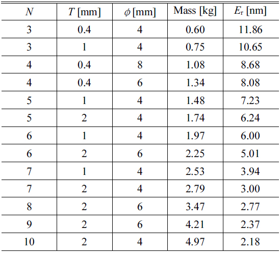
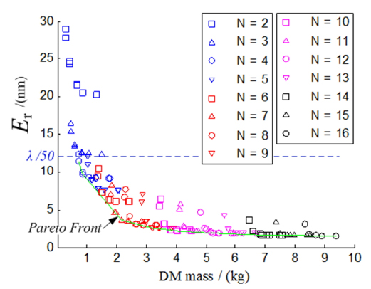
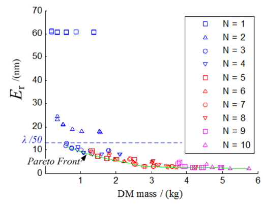
The triangularly configured DM is analyzed first. By fixing
[TABLE 5.] Pareto optimal designs for a triangularly configured DM
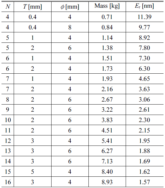
Pareto optimal designs for a triangularly configured DM
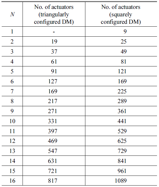
The relationship between
[TABLE 6.] Relation between N and the number of actuators

Relation between N and the number of actuators
Note that the parameter
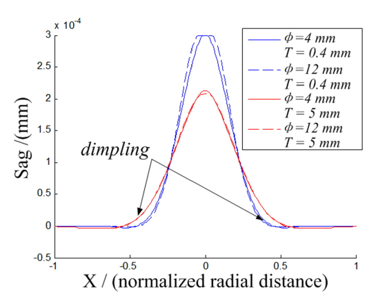
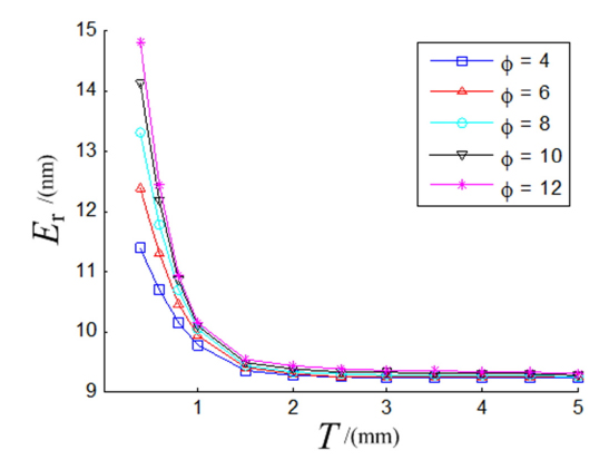
To examine the effects of parameters
5.2. Variation of Actuator Configuration
It has been believed that the triangularly configured DM is space-efficient in application and possesses higher performance than DMs with other kinds of actuator configurations. It seems that the triangularly configured DM is more suitable for the specific application discussed in this paper, since the WFE requiring correction comprises many trefoil WFEs. As another candidate, a squarely configured DM is analyzed. The trade space for the squarely configured DM is presented in Fig. 14. Similar trends can be found: The correction capability metric
[TABLE 7.] Pareto optimal designs for a squarely configured DM

Pareto optimal designs for a squarely configured DM
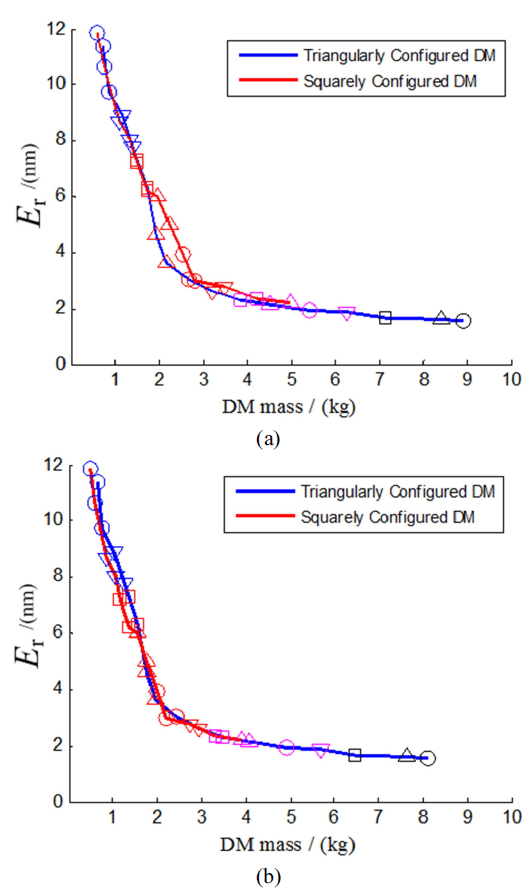
To compare the two different actuator configurations, only the two Pareto Fronts and Pareto Optimal Designs for each case are illustrated in Fig. 15(a). Accounting for the noncircular shapes of these two kinds of DM, a DM trimmed into a circle will lose some mass. Although the manner is rough, it can deliver some insights for application. The result for a trimmed DM is shown in Fig. 15(b). The difference between the two kinds of DM is relatively small, a squarely configured DM being slightly better than the triangularly configured one in Fig. 15(b). It can be explained by realizing that squarely configured DMs have more versatile changes in azimuthal order. However, since the difference is relatively small, it can be concluded that the type of configuration of DM is not a sensitive parameter in design; application and fabrication concerns take priority.
A parametric modeling method is introduced in this paper, making practical and flexible the design and optimization of DMs used in large-aperture optical systems. The parameter trade-off, which used to be impractical due to the time cost of manual-only meshing in large, complex models, is realized by a combination of manual meshing and autogeneration of FEM. Furthermore, the method is capable of dealing with other parametric modeling applications.
The metrics for a DM discussed in this paper are the correction capability and the mass of DM. The correction capability of a DM is represented by the residual WFE for specific figure correction, and the mass represents the launch cost concern. The optimal design has the best correction capability and the smallest mass. To find the interaction between variations of design parameters and the metrics of a DM, a full trade space is analyzed for triangularly and squarely configured DMs, providing design guidelines and insight. The results show that the correction capability of a DM increases as the mirror thickness