검색 전체 메뉴
PDF
맨 위로
OA 학술지
The Waveform Model of Laser Altimeter System with Flattened Gaussian Laser
  • 비영리 CC BY-NC
  • 비영리 CC BY-NC
ABSTRACT
The Waveform Model of Laser Altimeter System with Flattened Gaussian Laser
KEYWORD
Remote sensing , Laser altimeter , Flattened Gaussian beam , Waveform model , Generalized Gaussian
  • I. INTRODUCTION

    High resolution and accurate elevation of Earth or other planets can be acquired using space-borne laser altimeters. The range between the reference center on a satellite and the target surface is calculated by measuring the round-trip propagation time of short laser pulses, and other information such as surface roughness, slope, and reflectivity can also be measured through processing the received waveform. The Geoscience Laser Altimeter System (GLAS) on the Ice, Cloud and land Elevation Satellite (ICESat) with small footprint and along track spacing provided more accurate surface elevation and higher horizontal resolution on Earth observation, and was widely used to monitor ice sheet, sea ice, vegetation, and other changing environments [1-3].

    A Nd:YAG laser of fundamental mode was used in the GLAS system, and the cross section of the transmitted laser pulse satisfies a 2-dimensional Gaussian distribution, which means the majority of total energy focuses on the small central region, and decreases rapidly with the rising radius. Under this kind of energy distribution, the reflection of surface covering which locates on the center of the laser footprint will play a much bigger role in the received waveform. The energy distribution on the cross-section of a flattened Gaussian laser beam is more uniform than that of the fundamental mode, and the energy is nearly a constant in more than half of the total cross-section under the higher order beam. It is more suitable to detect the complex coverings of the Earth’s surface.

    Currently, the waveform model of fundamental mode laser used in GLAS was established by Gardner, Tsai, etc [4-6]. In this paper, the expressions of the main parameters of the laser altimeter waveform under flattened Gaussian laser were derived, and these results were used to compute total received energy, pulse width, variances of the propagation time delay and ranging error. A waveform simulator and parameter extraction program were used to verify the analytical expressions, which were universally used for both the flattened Gaussian beam and conventional fundamental mode ones. The effects of laser speckle, shot noise, and surface profile of the target were considered, and the influence of varying laser mode was quantitatively analyzed.

    II. FLATTENED GAUSSIAN BEAM

    For the fundamental mode laser, the laser cross-section and waveform of the transmitted laser pulse are both assumed to be Gaussian in shape:
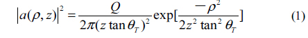
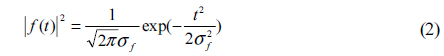
    image
    image

    Where ρ is the radius on the target surface measured from the center of the laser footprint, z is the altitude of the altimeter measured from target surface, Q is the total energy of the transmitted laser pulse, θT is the divergence angle of the laser beam, and σf is the pulse width of the transmitted laser pulse. For the fundamental mode lasers, the laser energy decreases rapidly as the radius increases, while for the high-order mode flattened Gaussian, the energy is nearly identical on the central cross-section of the laser footprint. According to the description of the reference [7, 8], the cross-section of a high-order mode flattened Gaussian beam can be represented as:

    image

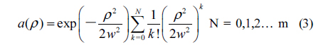
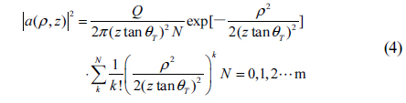
    According to Eq. (1), Eq. (3) is normalized processed, and is shown in Eq. (4).

    image

    III. ALTIMETER RECEIVED MODEL

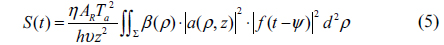
    The transmitted laser pulse undergoes Fresnel diffraction during propagation, and then it is reflected by the Earth’s surface. After another Fresnel diffraction, the incident laser light on the telescope is focused onto the photoelectric detector, and the received signal power is given by: [9]

    image

    η is the efficiency of the receiver optics and detector, AR is the area of the receiver aperture, Ta is one-way intensity transmittance of the atmosphere, hv is the energy of one signal photon, β(ρ) is the intensity reflection coefficient of the ground target, at ρ, and ψ is the time delay accounted for surface fluctuation and footprint reflection, where:

    image

    ξ(ρ) is the surface elevation, at ρ, and c is the light speed in a vacuum.

    The essential parameters of the received waveform consist of the expected number of detected signal photons denoted by N, the mean square width of the received pulse denoted by σs, the received signal time delay denoted by Ts, and the variance of Ts denoted by Var(Ts), which affect the total received energy, waveform shape, received pulse centroid, and the uncertainty of laser ranging, respectively.

    If we assume the reflection coefficient β(ρ) is a constant within the laser footprint, it can be denoted simply by β. If the target surface with fluctuant profile is quasi-flat with slope, and by generalizing the theory of Filin [10], the surface slope in the local level coordinate system should be converted into ‘modified surface slope’ φ in altimeter coordinate system, which is determined as a function of the satellite attitude, laser pointing and the surface slope itself. Then, N can be acquired by integrating signal power S(t) over t, and the integration result is:

    image

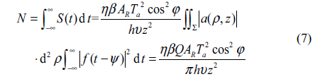
    Eq. (7) indicates that the received energy is irrelevant to transmitted laser mode, but related to transmitted laser energy, which means if the transmitted laser energy, the target surface, and the parameters of atmosphere and detector are the same, altering lasers from fundamental mode to flattened Gaussian does not actually change N.

    σs is expressed as the second-order normalized central moment, defined by: [9]

    image

    Ts can be calculated using Ts = 2z(1+tan2θT)/c. We substitute Eqs. (1), (4) and (5) into Eq. (8) to derive the expressions of mean square width of fundamental mode and flattened Gaussian laser, and the results are given by Eq. (9) and Eq. (10), respectively.

    image
    image

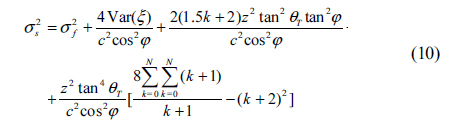
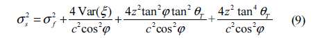
    In both Eq. (9) and Eq. (10), the received pulse widths are composed of 4 items. The transmitted pulse width is described as the first term, and the broadened effects produced by surface roughness of the ground target, modified slope, and the beam curvature are shown as the second, third and fourth terms, respectively. For a beam divergence of tens of μrad on a common laser altimeter system, the broadening effect of the last term is relatively weak and can be ignored. Actually, when the order in Eq.(4) is k = 0, which means flattened Gaussian laser changes to fundamental mode, Eq. (9) and Eq. (10) are identical, so Eq. (10) is common to both fundamental mode and flattened Gaussian laser.

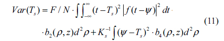
    According to the reference [9], the variance of Ts can be expressed in Eq. (11), and the first term caused by shot noise decreases as the signal energy increases, while the second term due to speckle can only be reduced by increasing Ks.

    image

    Ks is the ratio of the receiver area to the speckle correlation, and is usually called the speckle signal-to-noise ratio, given by Eq. (12). Where λ is the laser wavelength and F is the excess noise factor of the detector.

    image

    Under weak signal circumstances such as a space-borne laser altimeter system, shot noise is the dominant noise source. In Eq. (11), bn(p,z) is the normalized effective cross section of the laser beam.

    image

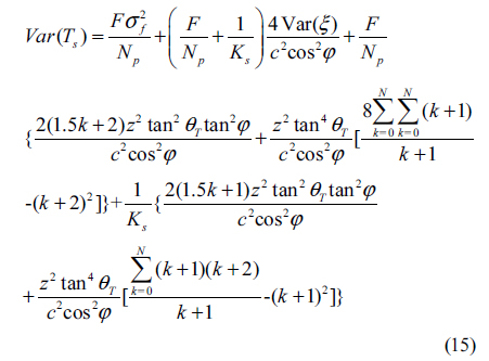
    By substituting Eqs.(1), (4) and (13) into Eq. (11) and integrating over ρ, the variance of Ts can be expressed as Eq. (14) for fundamental mode laser and Eq. (15) for flattened Gaussian laser. In addition, if the order is k = 0, the two expressions will be the same.

    image
    image

    As for the GLAS system, the satellite altitude is z = 600 km, the telescope diameter is d = 1 m, the laser wavelength is λ = 1064 nm, the divergence angle is θT = 110 μ rad, the transmitted energy of the laser is Q = 75 mJ, and the transmitted pulse width is σf = 2.37 ns. Then, Ks is nearly 106, which is considerably larger than N which is approximately 104, so the effect due to speckle can be ignored.

    IV. RESULTS

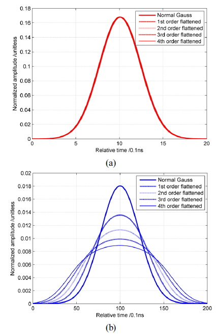
    According to the document related to the laser altimeter simulator given by NASA [11], the waveform simulator software was programmed in MATLAB codes, and was improved to run under a flattened Gaussian laser. The received waveform could be simulated by substituting the system parameters and assumed or actual surface profiles. Firstly, according to Eq. (1), the continuous laser waveform is discretized into a time series, and the sampling interval is 0.1ns typically. Then, as shown in Eq. (2) or (4), the cross section intensity of the transmitted beam is Gaussian or flattened Gaussian in the far-field, and on the target surface, the total energy of the incident beam is divided into a finite number of grids, 0.2 m × 0.2 m for a typical GLAS laser footprint. The reflected intensity and range delay are calculated independently for each grid, and the height and diffuse reflectivity can be specified independently for each grid on the surface profile. We use the GLAS system parameters as shown above, and set grid bin of surface profile to 0.2 m × 0.2 m and time bin to 0.1 ns, then the simulated waveforms are shown in Fig. 1.

    In Eq. (7), we proved that if the transmitted laser energy and measuring environment were kept the same, the laser mode would not affect the received laser energy. Consequently, in Fig. 1 the received laser energy of different laser modes were normalized. When modified slope is φ = 0 in Fig. 1 (a), which means normal incidence and flat surface with zero slope, the simulated waveforms are nearly the same in different modes of lasers, which corresponds well to the models in Eqs. (9) and (10). The reason is that the first two terms are the same, the third term influenced by slope is input by 0 slope, and the last term is relatively weak in simulation. When the slope is φ = 0.05, which is approximately 2.86°, the waveforms of flattened Gaussian with different orders are illustrated in Fig. 1 (b), and zero order is the same as for the fundamental mode laser. In the comparison of Fig. 1, increasing slope will decrease the amplitude of received waveform and broaden the pulse width severely, especially for higher-order flattened beams.

    0.05 is a typical slope in the icesheet region, because the slope of icesheet is slight in inland Antarctica, approximately ~1:1000, and increases from inland to coastal area. The surface slope is less than 1:300 in more than half of the total region, and is less than 3:200 in 90% of the total. [12] As shown in Fig. 1, the pulse widths broaden as the order of flattened Gaussian laser increases, whose trend agrees with Eq. (10), while the peak values of waveforms are inversely proportional to the order.

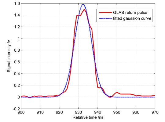
    In order to evaluate whether or not the simulated waveform precisely corresponds to the analytic expression shown as Eq. (10), we first should ensure that the pulse widths extracted from simulated waveforms are correct. So, one measured waveform by GLAS in Antarctica in March 2003 was chosen, illustrated in Fig. 2, to compare the main parameters given by NASA official GLA05 records and extracted by our waveform processing program based on the theory and method described in reference [6, 13]. In GLAS Algorithm Theoretical Basis Document, the transmitted and received waveform were treated as single Gaussian function or a sum of several, and the Gaussian parameters were extracted by Gaussian fit based on least squares algorithm.

    The transmitted width with σf = 2.72 ns (GLA05 i_parmTr) and received width with σs = 4.40 ns (GLA05 i_parm) were the same as the results extracted by our program. This waveform corresponded to the reflection from a very flat surface, which was typical of the Antarctica inland region. Then, we used the processing program to extract the pulse widths of the simulated waveforms which were illustrated in Fig. 1, and calculated the theoretical pulse widths according to Eq. (10). The comparisons between theoretical and simulated waveform widths under different order beams are listed in Table 1, and two groups of waveforms are drawn in Fig. 3.

    [TABLE 1.] Contrast between theoretical and simulated waveform widths under different order beams

    label

    Contrast between theoretical and simulated waveform widths under different order beams

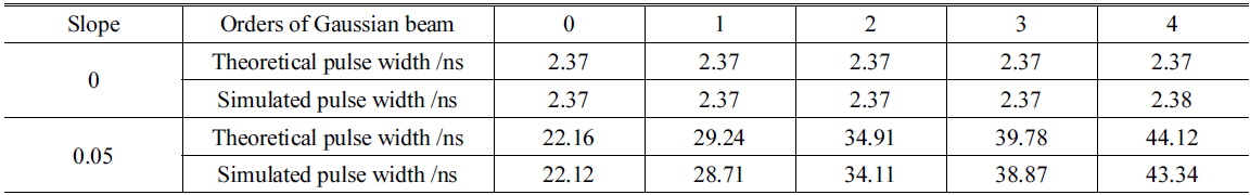
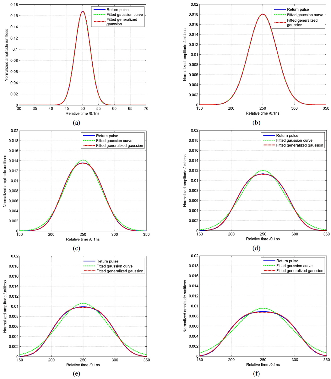
    As shown in Table 1, the simulated and theoretical pulse widths are nearly the same with all biases less than 1ns or 3%, which verifies the expression in Eq. (10). The comparison between Fig. 3 (a) and (b) shows that under the same laser of fundamental mode, the pulse width of waveform reflected by a flat surface is only about one-tenth than that of a surface with slope φ = 0.05, while the peak value is approximately ten times as high. Both shapes of waveform are Gaussian functions.

    The domains of coordinate axes in Fig. 3 (b)-(f) are the same. We can see clearly that the peak value decreases, the width increases as the order k ascends. From Table 1, the width under the condition of slope φ = 0.05 and order k = 4 is nearly twice that of slope φ = 0.05 and order k = 0.

    Besides, as the order
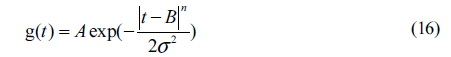
 k increases, the shape of waveform deforms, and cannot be supposed to be a strict Gaussian function in Fig. 3 (b)-(f). We use the generalized Gaussian function, shown in Eq. (16), to fit these waveforms, and the new fitted shapes illustrated in Fig. 3 (a)-(f) by red dash lines.

    image

    Where A is the amplitude, B is the center of Gaussian function, n is the power of generalized Gaussian function and σ is the generalized Gaussian width. As we can see in Fig. 3, compared to Gaussian function fit, the generalized Gaussian model significantly improves the fit results. Generalized Gaussian fittings influence the amplitude A in Eq. (16) slightly, however, as shown in Table 2, owing to the rising of n in Eq. (16), which serves as the power parameter, the widths increase drastically as the beam order rises. And, the derivation process in this paper is irrelevant to the generalized Gaussian function, so the physical interpretation needs to be researched in the future.

    [TABLE 2.] Parameters fitted by generalized Gaussian model

    label

    Parameters fitted by generalized Gaussian model

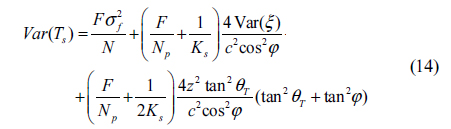
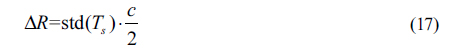
    When laser ranging is based on the time of flight, the ranging error or ranging precision arising from the laser itself and the target will be the product of uncertainty of timing and half of the velocity of light, and it can be expressed in Eq. (17), where ‘std’ means standard deviation.

    image

    We substitute N, derived in Eq. (7), into Eqs. (15) and (17). As analyzed above, the shot noise serves as the primary effect in the space-borne laser altimeter system, so after simplification we get the expression for ranging error.

    image

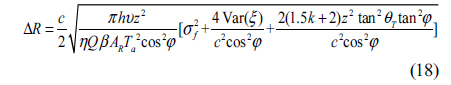
    If we assume atmospheric transmittance is Ta = 0.7, detector efficiency is η = 0.5, excess noise factor is F = 5, reflection coefficient is β = 0.3, the expected photons will be N = 20478, which is approximately 3.83 fJ and agreed with the result given in reference [14]. Under any orders of flattened Gaussian lasers, when slope is φ = 0, the ranging error will be less than 1 cm and can be nearly ignored. However, under 0-4th beam orders, when slope is φ = 0.05, it will become 5.2 cm, 6. 8cm, 8.2 cm, 9.3 cm and 10.3 cm, respectively. Consequently, the ranging error also increases with the rising of mode order k and slope φ, and if the slope is φ = 0.05, the error of the 4th order flattened Gaussian laser will be twice than that of fundamental mode laser.

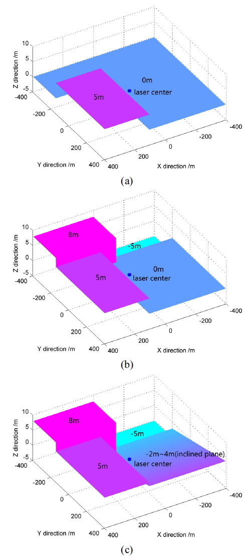
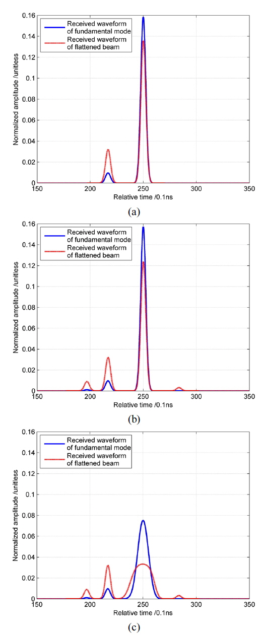
    In the above content, all the targets are assumed to be a single quasi-flat surface, however, the actual target would be much more complicated. As a result, if we assume that there are two quasi-flat surfaces on the target, which is shown in Fig. 4 (a) and can be considered as a building with 5m height on the ground. In Fig. 5 (a), the simulator shows the corresponding waveforms of fundamental mode and 4th order flattened beam. Then, we assume that there are two buildings with different heights and a pit on the ground, shown in Fig. 4 (b), and finally the ground is changed to be an inclined plane with 0.01 slope, shown in Fig. 4 (c). As for GLAS parameters, the divergence θT is equal to 110 μrad, which means that more than 99% of laser energy locates within a 200 m radius circle.

    The transmitted laser energies are the same, and we can clearly find that the flattened beam get much better performance for a multi-surface target. In Fig. 5 (a), both lasers indicate that there are two surfaces on the target, but the first waveform peak of fundamental mode with approximately 0.01 amplitude, which corresponds to the 5 m height building, is much less than that of flattened beam with over 0.03 amplitude. And the time interval between two peaks of waveform could invert the distance of two surfaces of target. In Fig. 5 (b) and 5 (c), when the areas of new surfaces become smaller and further from the laser center, we can hardly recognize the corresponding peaks in waveform, and the last peak of the fundamental mode has completely disappeared. The reason is that the energy of the fundamental mode decreases rapidly with the radius of laser footprint rising, while flattened Gaussian laser beam is more uniform than that of fundamental mode and can reflect the effects of target surface far from the laser center.

    Although the ranging error of flattened Gaussian beams is bigger than that of the fundamental mode, typically for 10.3 cm under 4th order compared to less than 1 cm with 0.05 slope, the flattened beams could detect more details of the target. And if the surface is flat without slope, the ranging error is the same under flattened Gaussian beams and the fundamental mode. Besides, the derived ranging error expression in this article is arising from the laser itself and the target, which is only part of the total ranging error, and another main influencing factor is pointing errors, 1.5″ of which makes 21.8 cm ranging error with 0.05 slope for typical GLAS parameters [15, 16]. According to law of error propagation, the total ranging error is equal to the root of the sum of every error squared.

    V. CONCLUSION

    The main parameters of received pulse under flattened Gaussian laser were derived and verified through waveform simulator and processing, and the bias between simulated and theoretical pulse widths were less than 3%. These new expressions of flattened Gaussian laser were universal compared to the former fundamental mode, and could be used not only under flattened Gaussian lasers but also fundamental mode when the order was set to be zero.

    Both the pulse width and ranging error increase as the modified slope and flattened Gaussian order grow; therefore, laser altimeter will get more accurate ranging performance under small nadir angles, meaning nearly normal incidence, and small surface slope. As for received waveform of higher order flattened Gaussian, the shape deforms and is no longer a strict Gaussian function, because the incident energy of laser footprint does not satisfy 2-dimensional Gaussian distribution. Generalized Gaussian model was used to express these curves and got very good fit results, and the physical interpretation of generalized Gaussian model needs to be researched in the future.

    The flattened beam got much better performance under the circumstance of multi-surface target, especially when the small surface is far from the center of the laser footprint, and it is more suitable to detect the complex coverings of the Earth’s surface. In addition, the established expressions and waveform simulator are meaningful to the system design of the flattened Gaussian laser altimeter.

참고문헌
  • 1. Schutz B. E., Zwally H. J., Shuman C. A., Hancock D., DiMarzio J. P. 2005 “Overview of the ICESat mission,” [Geophys. Res. Lett.] Vol.32 P.L21S01-1-4 google
  • 2. Hilbert C., Schmullius C. 2012 “Influence of surface topography on ICESat/GLAS forest height estimation and waveform shape,” [Remote Sensing] Vol.4 P.2210-2235 google cross ref
  • 3. Kwok R., Cunningham G. F., Manizade S. S., Krabill W. B. 2012 “Arctic sea ice freeboard from IceBridge acquisitions in 2009: Estimates and comparisons with ICESat,” [J. Geophys. Res.] Vol.117 P.C02018-1-14 google
  • 4. Gardner C. S. 1992 “Ranging performance of satellite laser altimeters,” [IEEE T. Geosci. Remote Sensing] Vol.30 P.1061-1072 google cross ref
  • 5. Tsai B. M., Gardner C. S. 1983 “Remote sensing of sea state using laser altimeters,” [Appl. Opt.] Vol.21 P.3932-3940 google
  • 6. Brenner A. C., Zwally H. J., Bentley C. R., Csatho B. M., Harding D. J., Hofton M. A., Minster J.-B., Roberts L., Saba J. L. 2011 Derivation of Range and Range Distributions from Laser Pulse Waveform Analysis for Surface Elevations, Roughness, Slope, and Vegetation Heights, AS Algorithm Theoretical Basis Document Version 5.0 google
  • 7. Gori F. 1994 “Flattened Gaussian beams,” [Opt. Commun.] Vol.107 P.335-341 google cross ref
  • 8. Cerjan A., Cerjan C. 2010 “Analytic solution of flat-top Gaussian and Laguerre-Gaussian laser field components,” [Opt. Lett.] Vol.35 P.3465-3467 google cross ref
  • 9. Gardner C. S. 1982 “Target signatures for laser altimeters: an analysis,” [Appl. Opt.] Vol.21 P.448-453 google cross ref
  • 10. Filin S. 2003 “Recovery of systematic biases in laser altimetry data using natural surfaces,” [Photogramm. Eng. Rem. S.] Vol.69 P.1235-1242 google cross ref
  • 11. Abshire J. B., McGarry J. F., Pacini L. K., Blair J. B., Elman G. C. 1994 Laser Altimetry Simulator, User’s Guide Version 3.0 google
  • 12. Brenner A. C., DiMarzio J. P., Zwally H. J. 2007 “Precision and accuracy of satellite radar and laser altimeter data over the continental ice sheets,” [IEEE T. Geosci. Remote Sensing] Vol.45 P.321-331 google cross ref
  • 13. Ma Y., Li S., Zhou H., Zheng G. 2012 “Noise suppression method for received waveform of satellite laser altimeter based on adaptive filter,” [Infrared and Laser Engineering] Vol.41 P.3263-3268 google
  • 14. Fricker H. A., Borsa A., Minster B., Carabajal C., Quinn K., Bills B. 2005 “Assessment of ICESat performance at the salar de Uyuni, Bolivia,” [J. Geophys. Res.] Vol.32 P.L21S06-1-5 google
  • 15. Luthcke S. B., Carabajal C. C., Rowlands D. D. 2002 “Enhanced geolocation of spaceborne laser altimeter surface returns: parameter calibration from the simultaneous reduction of altimeter range and navigation tracking data,” [J. Geodyn.] Vol.34 P.447-475 google cross ref
  • 16. Luthcke S. B., Rowlands D. D., Stoneking E. 2000 “Spaceborne laser-altimeter-pointing bias calibration from range residual analysis,” [J. Spacecraft Rockets] Vol.37 P.374-384 google cross ref
OAK XML 통계
이미지 / 테이블
  • [ ] 
  • [ ] 
  • [ ] 
  • [ ] 
  • [ ] 
  • [ ] 
  • [ ] 
  • [ ] 
  • [ ] 
  • [ ] 
  • [ ] 
  • [ ] 
  • [ ] 
  • [ ] 
  • [ ] 
  • [ FIG. 1. ]  Simulated waveforms of flattened Gaussian with different orders. (a) Surface with 0 slope; (b) Surface with 0.05 slope.
    Simulated waveforms of flattened Gaussian with different orders. (a) Surface with 0 slope; (b) Surface with 0.05 slope.
  • [ FIG. 2. ]  The actual waveform and processed result of GLAS.
    The actual waveform and processed result of GLAS.
  • [ TABLE 1. ]  Contrast between theoretical and simulated waveform widths under different order beams
    Contrast between theoretical and simulated waveform widths under different order beams
  • [ FIG. 3. ]  The contrast of original, fitted Gaussian, and fitted generalized Gaussian waveforms with different slopes and beam orders. (a) Modified slope with φ=0 and beam order with k=0; (b)-(f) Modified slope with φ=0.05 and beam orders with k=0, 1, 2, 3, 4.
    The contrast of original, fitted Gaussian, and fitted generalized Gaussian waveforms with different slopes and beam orders. (a) Modified slope with φ=0 and beam order with k=0; (b)-(f) Modified slope with φ=0.05 and beam orders with k=0, 1, 2, 3, 4.
  • [ ] 
  • [ TABLE 2. ]  Parameters fitted by generalized Gaussian model
    Parameters fitted by generalized Gaussian model
  • [ ] 
  • [ ] 
  • [ FIG. 4. ]  Laser footprint illuminating different target surfaces. (a) Target with two flat planes; (b) Target with four flat planes; (c) Target with three flat surfaces and an inclined planes.
    Laser footprint illuminating different target surfaces. (a) Target with two flat planes; (b) Target with four flat planes; (c) Target with three flat surfaces and an inclined planes.
  • [ FIG. 5. ]  Received waveform of different target surfaces (a) Waveforms corresponding to two flat planes; (b) Waveforms corresponding to four flat planes; (c) Waveforms corresponding to three flat surfaces and an inclined planes.
    Received waveform of different target surfaces (a) Waveforms corresponding to two flat planes; (b) Waveforms corresponding to four flat planes; (c) Waveforms corresponding to three flat surfaces and an inclined planes.
(우)06579 서울시 서초구 반포대로 201(반포동)
Tel. 02-537-6389 | Fax. 02-590-0571 | 문의 : oak2014@korea.kr
Copyright(c) National Library of Korea. All rights reserved.