The human eye is typically capable of detecting light at wavelengths between 400 and 700 nm, a range known as the visible band. The human eye contains photoreceptors with three kinds of color-sensitive pigments for absorbing energy in this wavelength range, thereby enabling the eyes to see [1]. Without the presence of light, the colors as well as the shapes of objects in the scene being observed would disappear.
The development of infrared imaging technology has provided us with night vision, which is the ability to see in conditions of low light or total darkness. Although night vision devices were previously only used by military forces, they have since become more widely available for civilian use. Night vision technologies can be divided into three main categories: low-light imaging, thermal imaging and nar-IR illumination, each of which has its advantages and disadvantages. A popular and sometimes inexpensive technique for achieving night vision uses a device that is sensitive to invisible near-IR radiation in conjunction with a near-IR illuminator. This technique can be performed by most cameras, because their sensors can detect near-IR wavelengths. However, the resulting scene appears as a monochrome image containing single-color or false-color tones which do not correspond to everyday experiences [2, 3]. Therefore, humans experience monochrome images as highly unnatural.
Furthermore, in situations in which it is critical to obtain color information, such as for accurate identification or tracking purposes, a color image is much more advantageous than a monochrome image. Over the past 20 years, much research has been devoted to producing true-color images from near-IR imaging. The main focus of these studies involves the fusion of visible and infrared images, a technique for which the results are promising when the corresponding day-time images are available [4-9]. Meanwhile, attempts to produce color images by using only infrared light have led to the development of various applications in which a set of three sensors that are individually sensitive to different wavelengths in the near-IR band are used. For example, a new night vision camera with a set of three near-IR sensors was recently developed by AIST (the National Institute of Advanced Industrial Science and Technology in Japan) [10]. It has been reported that this camera can record clear, high-frame-rate color videos even in darkness, and can reproduce colors that are equivalent or similar to the colors of the same objects under visible light. However, even though the assessment data for the color accuracy has not yet been released, the examples presented by AIST indicate that an improvement in the color signal processing method is required.
This paper proposes an algorithm to recover the colors of objects from multiple near-IR images. The key point is to use the information from the reflectance curve in the wavelength range from 700 to 900 nm, which is near the red edge of the visible band. In Section II, the proposed algorithm is described with the aid of a flowchart. The International Commission on Illumination (CIE) color coordinates
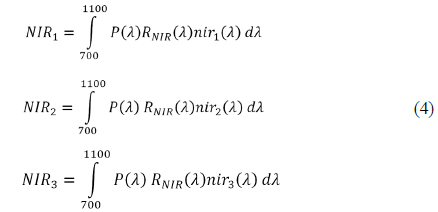
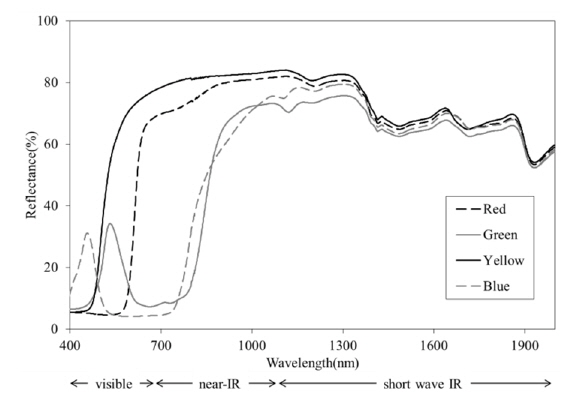
Figure 1 shows an example containing the reflectance curves for four color patches painted with red, green, yellow, and blue paint, respectively. According to the definitions that are used in night vision technology [12], the visible band is considered to include wavelengths ranging from 400 to 700 nm, the near-IR region is defined to include wavelengths between 700 and 1100 nm, whereas IR wavelengths longer than 1100 nm are defined as the shortwave IR band that is useful for the detection of objects in a scene.
Figure 1 presents several noteworthy features. The reflectance curve in the visible band has a particular structure that depends on color. However, in the near-IR band, the reflectance curves of the four colors tend to converge to gradually become identical throughout the shortwave IR band. This behavior has been observed for many different materials [13].
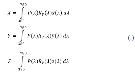
The reflectance curve in the visible band is particularly important since it uniquely describes the color of the object as perceived by human observers. In 1931, the CIE created the CIE

where,
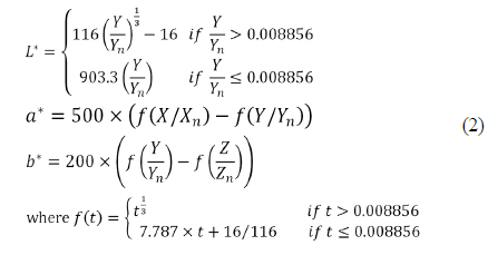
In 1976 the CIE

where

The reflectance curve in the near-IR band does not contribute to defining the color in terms of

where, P(
where
Before the proposed recovery algorithm is presented, a simple combination commonly used in remote sensing applications is considered [15]. The values
The aim of the proposed algorithm is to recover the CIE color coordinates of objects from a series of gray images captured under three spectral near-IR illuminations. This can be achieved using the polynomial regression of the form [16]

where and are the vector forms of the CIE color coordinates

The accuracy of
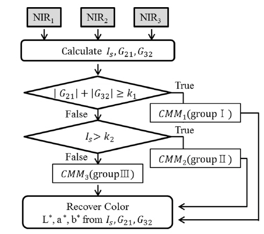
To improve the recovery performance, the proposed algorithm is designed to acquire an individual
In order to classify the highly correlated colors together, a new set of parameters is derived from the near-IR tristimulus value
In Eq. (8), Is means the height of the reflectance curve
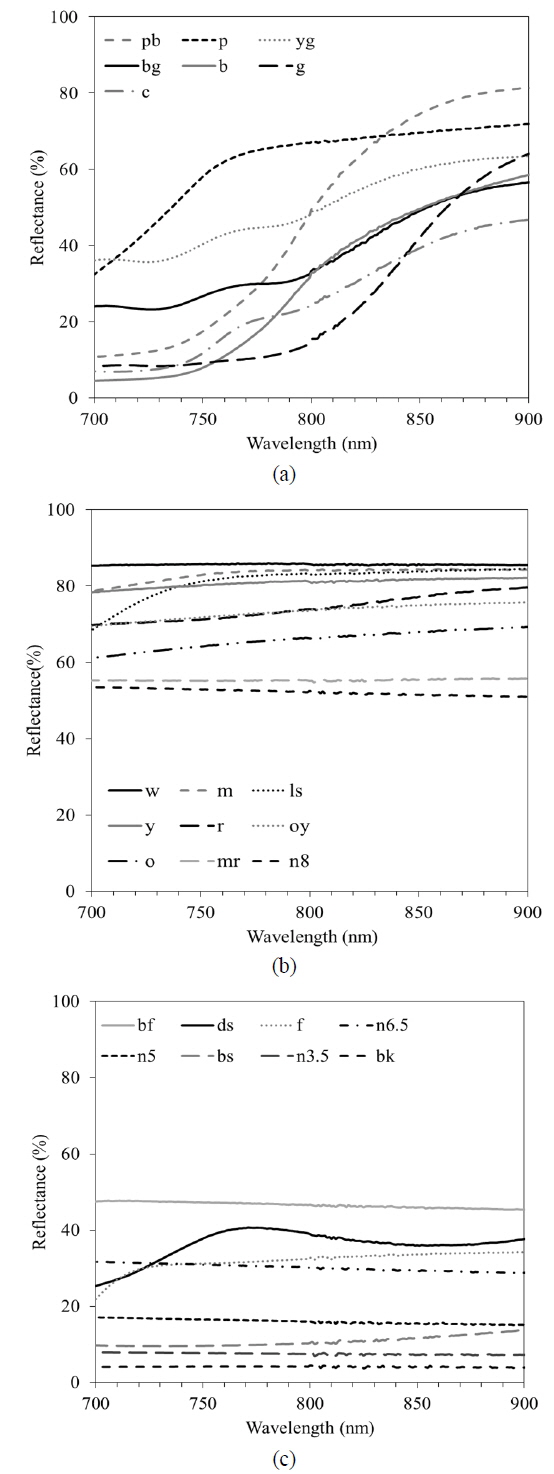
As can be seen in Fig. 1, selected reflectance curves in the near-IR band exhibit steep gradients, while others display gentle gradients. In this study, each set of target colors is classified into two groups based on the gradient of the reflectance curve, following which the gentle gradient group is additionally classified into two further groups based on the height of the reflectance curve. The workflow shown in Fig. 2 consists of three paths. If the sum of|

where and are the vector forms of
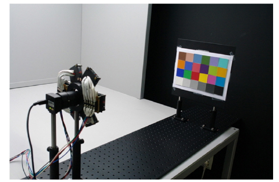
The experiment is carried out in dark condition. The experimental room (including the ceiling and the wall) is painted matte black. The experimental configuration is presented in Fig. 3. A screen that is attached to the target color objects is placed 0.7 m from a multiple spectral near-IR illuminator. Through the hole in the center of the illuminator, a monochrome digital camera is placed facing the screen as shown in Fig. 3. The camera has an image sensor consisting of a diagonal 1/3 inch CCD array with 1.25 M effective pixels. Its spectral response ranges from 300 to 1000 nm, and the maximum sensitivity is near 580 nm. Using the camera’s software, automatic white balance function and a gamma value are set to ‘off’ and 1, respectively. The 16-bit data of the captured image is saved in TIFF format.
Details of the illuminator and target color objects are described in the following sections.
3.1. Multiple Spectral Near-IR Illuminator
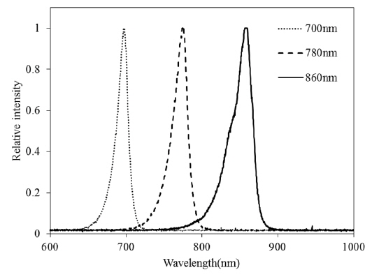
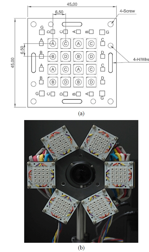
The multiple spectral near-IR illuminator consisting of six near-IR LED array modules is custom-designed. Figure 4 (a) shows a schematic diagram of one of the six modules. In the diagram, Ⓐ, Ⓑ, Ⓒ, and Ⓓ indicate four types of near-IR LEDs with peak wavelengths at 700, 740, 780 and 860 nm, respectively. Each module consists of a uniform arrangement of four of each of these types, i.e., a total of 16 LEDs per module. Figure 4 (b) shows the assembled multiple spectral near-IR illuminator with the six modules, which are slightly tilted toward the central hole in the form of a sunflower. The luminous intensity of the LEDs in all six modules is controlled according to type by using four separate power supplies. For the experiment, the three types of LEDs with peak wavelengths at 700, 780 and 860 nm were selected.
Figure 5 presents the spectral power distributions of these three types of LEDs as measured by using a USB-650 spectrometer. In Fig. 5,
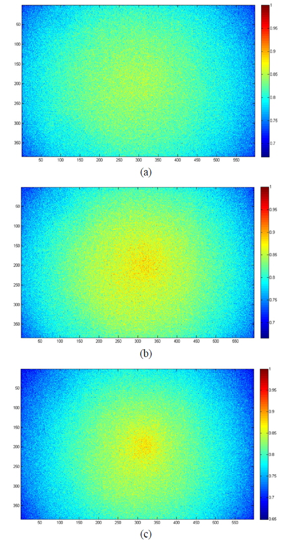
The spatial uniformity of the custom-designed illuminator was measured by using a uniform gray card (X-rite ColorChecker Custom White Balance Card, of which the size of the square, excluding the border, is 27.4 × 17.8 cm). In Figure 3, the white balance card is attached to the screen. Figure 6 shows the captured images of the white balance card. The uniformity of the entire plane is shown at a glance in Fig. 6 (a), (b), and (c), in which the resultant color-coded images that were obtained under the illumination of
In addition, the pixel positions of each of the images in Fig. 6 correspond to the size of the gray card (27.4 × 17.8 cm). All three of the color-coded images display concentric rings of which the color gradually changes, and in which the maximum code value is 1 near the center. Toward the edges of the gray card, the code value is gradually reduced to about 0.7 in the center of the x-axis and 0.8 in the center of the y-axis. Comparing the three images in Fig. 6, the degree of non-uniformity of
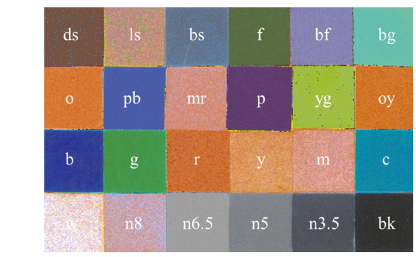
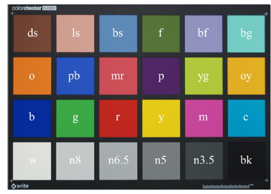
The ColorChecker is generally used as a color calibration target in visible imaging technology. It includes 24 color patches in a 6 × 4 grid, each slightly under 2 inches square, made of matte paint applied to smooth paper, and surrounded by a black border. A photograph of the ColorChecker is shown in Fig. 7, in which the original colors as they appear in visible light are shown. Six of the patches form a uniform gray lightness scale; white (w), neutral 8 (n8), neutral 6.5 (n6.5), neutral 5 (n5), neutral 3.5 (n3.5), and black (bk). Another six patches represent the primary colors; red (r), green (g), blue (b), cyan (c), magenta (m), and yellow (y). The remaining colors include approximations of natural colors, such as human skin tones (ds and ls), blue sky (bs), a typical leaf (f), a blue chicory flower (bf), and bluish green (bg). The remaining colors were chosen arbitrarily to represent a gamut: orange (o), purplish blue (pb), moderate red (md), purple (p), yellow green (yg), and orange yellow (oy). The letters in parentheses represent the acronym for each tone.
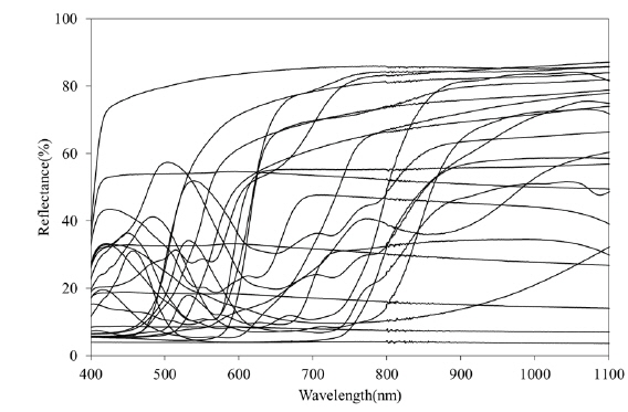
The spectral reflectance of each patch was measured by using a Cary 5000 UV-Vis-NIR spectrophotometer after cutting the 24 patches from the ColorChecker. Figure 8 shows the accumulated reflectance curve for all 24 patches in the wavelength range from 400 to 1100 nm, which includes both the visible and the near-IR bands. As expected, based on the explanation in Fig. 1, the reflectance data shows the inherent structure of each color in the visible band (400~700nm). In the near-IR band, the reflectance data increases near the red edge of the visible band (700~900 nm) before assuming a uniform appearance. As the red edge of the visible band is approached (Fig. 8), the reflectance data of some colors increase rapidly and their reflectance curve displays a steep gradient, whereas other colors have a gentler gradient. Using the measured spectral reflectance data in the visible band, it is possible to calculate the
[TABLE 1.] The X, Y, Z values for Illuminants D65 and the derived L* , a* , b* values of 24 patches
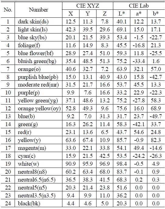
The X, Y, Z values for Illuminants D65 and the derived L* , a* , b* values of 24 patches
As shown in the experimental setup, the 24 cut patches were rearranged in the form of a 6 × 4 grid without the black borders to prepare them for use as target color objects. The target object was created to have the same size as the gray card that is shown in Fig. 6 to compensate for non-uniformity in illumination.
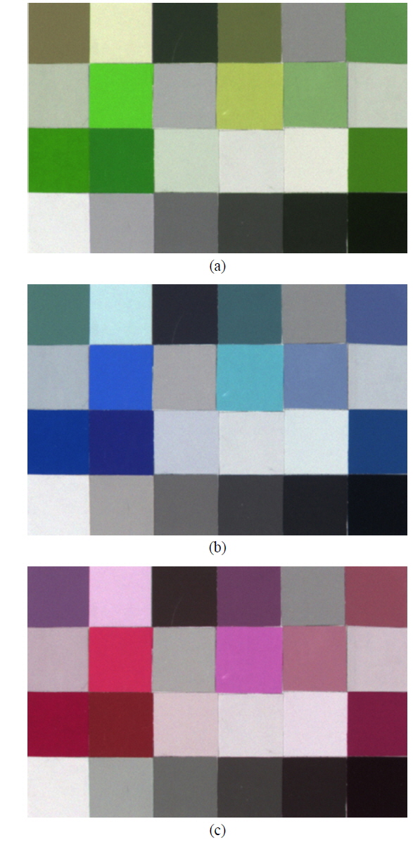
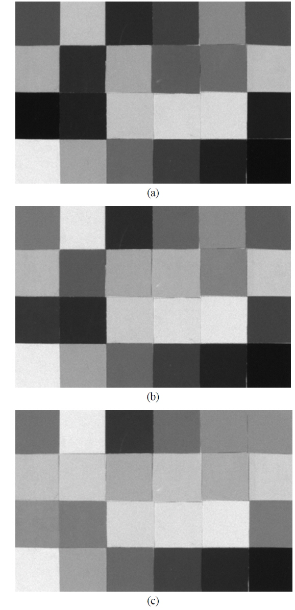
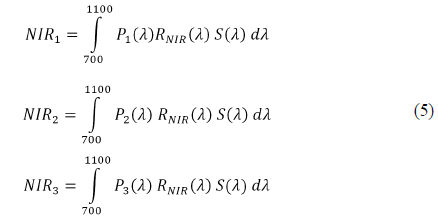
Figure 9 shows a set of monochrome images, after compensation for non-uniformity, that was experimentally obtained from the target color objects. Figure 9 (a), (b), and (c) show the results of illumination at
Figure 9 was used to define the set of tristimulus values
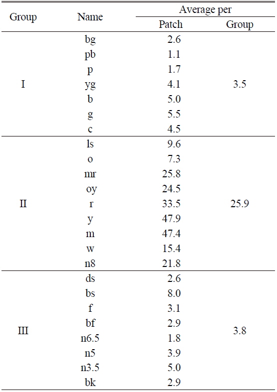
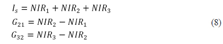
Figure 11 shows a color image that was recovered from the three near-IR images in Fig. 9 by using the proposed algorithm. The 24 patches are classified into three groups on the basis of the criteria suggested by the proposed algorithm using MATLAB. Figure 12 (a), (b), and (c) illustrate the reflectance curves from 700 to 900 nm of the color patches belonging to groups I, II, and III, respectively. The bluish or greenish patches, all of which have a steep gradient, are included in group I, whereas the reddish or yellowish patches, which have a gentle gradient and a large reflectance sum, are included in group II. The remaining patches, which have a gentle gradient and a small reflectance sum, are included in group III. The individual color mapping matrix
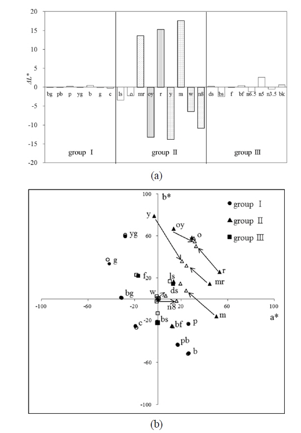
At a glance, the colors in Fig. 11 appear very similar to those of the original patches. However, some colors differ significantly from the original. The color difference
[TABLE 2.] The color difference between original and recovered colors

The color difference between original and recovered colors
The average color difference
An algorithm to recover the colors of objects from multiple near-IR images is proposed. The CIE color coordinates
In the next study, a feasibility test will be continued for an extended number of color patches using the other Color Rendition Chart, for example 169 colors made of matte paint of the ColorChecker DC. Near-IR reflectance behavior of artifacts and natural objects made of various materials also should be investigated in further research. In addition, the spatial uniformity of the illuminator could be enhanced by improving the optical design of components, such as the lens, and the beam shaping diffuser [21]. It is expected that multiple-spectral illuminations provided by an illuminator with a narrow half-width, such as a laser, used in conjunction with a high-resolution camera, would be helpful to enhance the color image quality.