In this study, a novel parallel wavefront correction system architecture is proposed, and a model-based tabu search (MBTS) algorithm is introduced for this new system to compensate wavefront aberration caused by atmospheric turbulence in a free-space optical (FSO) communication system. The algorithm flowchart is presented, and a simple hypothetical design for the parallel correction system with multiple adaptive optical (AO) subsystems is given. The simulated performance of MBTS for an AO-FSO system is analyzed. The results indicate that the proposed algorithm offers better performance in wavefront aberration compensation, coupling efficiency, and convergence speed than a stochastic parallel gradient descent (SPGD) algorithm.
Recently free-space optical (FSO) communication has attracted more and more attention as it becomes widely used among the telecommunication community for both ground- and space-based wireless links and “last-mile” applications [1], due to its unregulated spectrum, high potential bandwidth, relatively low power requirement, low bit error rate, and ease of redeployment. However, phase disturbances from atmospheric turbulence along propagation paths, manifesting as intensity fluctuation (scintillation), beam wandering, and beam broadening at the receiver all lead to significant decrease of coupling efficiency [2], which seriously influences the stability and reliability of FSO communication systems [3].
An adaptive optical (AO) system is an effective method to improve laser-beam quality by correcting any wavefront aberration, and has already allowed great achievements [4-9]. Generally, in a conventional AO system a Shack-Hartmann wavefront sensor (S-H sensor) [10] measures the optical phase deviations of an incoming wavefront, and a deformable mirror (DM) is used to compensate for the phase distortion. Then the DM generates a wavefront phase to compensate for the phase aberration based on phase-conjugation theory [11, 12].
Under strong scintillation, sensorless AO systems are proposed to compensate for the wavefront aberration. Some very effective blind control optimized algorithms, such as stochastic parallel gradient descent (SPGD) and simulated annealing (SA) have been proposed to improve the performance of the FSO system [13]. In this study, a new method called the model-based tabu search (MBTS) algorithm is proposed to offer better performance in atmospheric turbulence compensation. Tabu search (TS) is a meta-heuristic random-search algorithm [14] that starts from an initial solution and selects some specified directions for probing. To avoid being trapped in a local minimum, TS uses a flexible method to record the process of optimization and selection to guide the next search step, while a Zernike model-based (MB) method in an AO system can decrease the dimension of the search space, relieve calculation complexity and accelerate convergence speed. Model-based tabu search (MBTS), the combination of MB and TS approaches, will benefit from these two methods and perform better in an FSO system, since it can effectively improve coupling efficiency at the receiver and reduce energy loss in the laser propagation path. Most important is that MBTS uses very few iterations, far less than does SPGD (which usually needs hundreds of iterations). Moreover, to further improve the performance of the MBTS algorithm, a novel parallel correcting system is proposed. The newly invented system can increase the speed of correction of the wavefront aberration by simply combining several uniform AO subsystems together, each subsystem correcting certain orders of aberration by MBTS. The working principle of this new system is explained further.
This paper is organized as follows: Section 2 provides models of an FSO communication system, sensorless AO system, and DM. Section 3 gives an analysis of MBTS algorithm and its working principles in the FSO communication system, as well as a simple and novel hypothetical design for a parallel correcting system with multiple AO subsystems. In Section 4, some simulations are carried out to show the performance of the proposed MBTS in a sensorless AO-FSO system, in comparison with SPGD algorithm. Finally, some conclusions from this study are given in Section 5.
2.1. FSO Communication System with Model - Based Tabu Search Algorithm
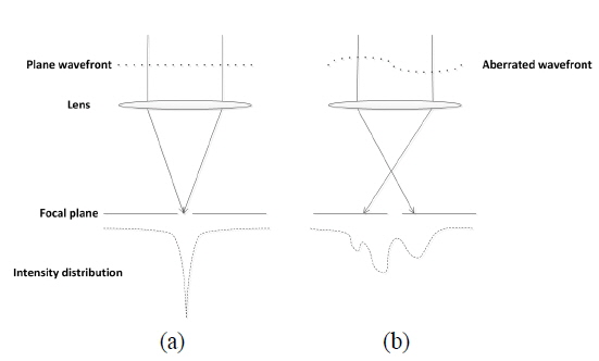
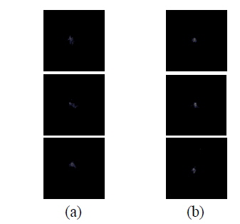
A laser communication system in atmospheric turbulence works poorly, because an aberrated wavefront leads to energy loss in receiver. In an ideal case when the system does not introduce any aberration to the laser signal, all fluorescence is emitted from a point, so that the laser is well coupled to a single mode fiber (see Fig. 1 (a)). When atmospheric turbulence is present, the intensity in the focal plane depends on the wavefront of incident light, which spreads widely over the focal plane of lens due to the wavefront aberration; thus the coupling efficiency at the receiver will degrade, and the bit error rate will increase (Fig. 1 (b)) [15].
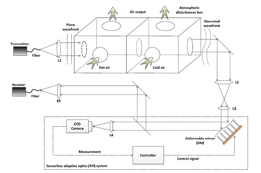
The simple schematic diagram of an FSO experimental setup is illustrated in Fig. 2. A laser from a distant source passes through an atmospheric disturbances box, in which the wavefront is disturbed by the atmospheric turbulence device. In a conventional AO system, when the laser enters it is reflected by a deformable mirror (DM) and directed to a wavefront sensor (WFS). The measured signal is sent to a controller to reconstruct the wavefront from the WFS measurement, and to compare the reconstructed wavefront to a reference plane wavefront for computation of the control signal for the DM. Consequently, the DM deforms its surface to counteract the wavefront aberration. In this way the laser wavefront is compensated, and thus the coupling efficiency in the communication receiver increases. However, in a recently proposed sensorless AO system, a CCD camera replaces the WFS. This camera measures the intensity at the focus plane to obtain a performance metric and generate a good control signal vector. In addition, a good algorithm should also provide a better solution in fewer iterations for a real-time system in practice.
Our goal is to find a control signal so that the DM can generate the best surface deformation to compensate for the wavefront aberration, so that in turn more laser energy is coupled into the single mode fiber.
2.2. Wavefront Compensation Device
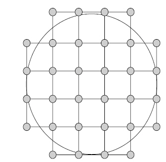
In general, a DM with more actuators could generate a more precise correcting phase to compensate for lower-order but higher-value aberration. However, a DM with too many actuators and too large a receiving aperture is not useful in laser transmission, because it requires reshaping of the laser beam to a large diameter to match the receiving aperture. In our analysis, a DM with 32 actuators is a suitable selection that generates an acceptable result and has no excessive requirement for beam reshaping. The normalized layout of the 32-element DM actuators is shown in Fig. 3.
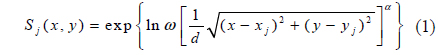
We approximate the DM influence function by a Gaussian mdel as follows:

where

where
2.3. Model-based Compensation in Adaptive Optics
From the conventional point of view, we often pay lot of attention to the control voltages applied to the actuators, but problems occur due to a solution space of high dimension, which can result in slow convergence, large computational burden, and unsatisfied convergence value of the control algorithm, since increasing the number of actuators brings a geometric increase in the number of calculations of the control solution. This is important for real-time performance of the system. A new, alternative approach is to use a Zernike model to fit induced wavefront aberration and to indirectly get appropriate voltages, instead of directly using a DM model. No matter how many actuators exist, we only need to obtain the linear relationship between the control voltages and Zernike coefficients, so that the number of calculations will decrease, which is better for an FSO system under high-speed workload.
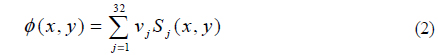
We assume the wavefront aberration
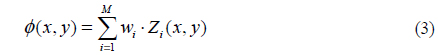
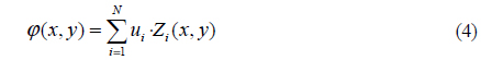
In other words, the aberration of the incident wavefront
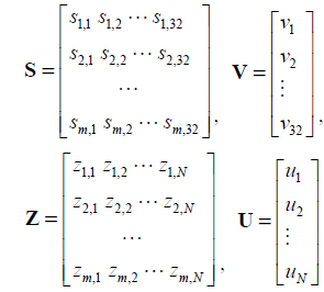
In practice, the correcting aberration

where

and

where S† is the pseudo-inverse of S. Obviously it can be calculated offline and is simplified; what we need to do is simply find the best U = (
2.4. Parallel Wavefront Correcting System
The sensorless AO system described above cannot take the speed of the proposed algorithm to the extreme, so here we put forward a new system architecture that combines many uniform AO subsystems, to increase the processing rate.
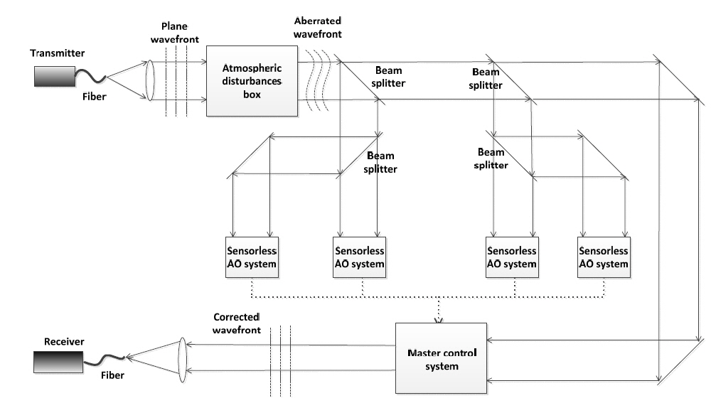
We outline a simple conception of this equipment with four AO systems based on the algorithm proposed in this paper, as examplified in Fig. 4. The incident light is divided into some number of parts by beam splitters. Each part of light passes through a sensorless AO subsystem and is corrected by the MBTS algorithm: AO subsystem I gets the best solution (
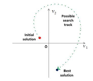
The tabu search (TS) algorithm is an effective way to find an optimal or nearly optimal global solution, which can guide the search process to avoid a local optimum and find the global optimum. The TS algorithm begins with an initial solution
In general, the TS algorithm selects a new solution according to a rule such as this: If the new
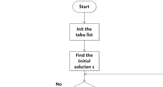
The detailed process is described as follows:
(1) Select an initial solution. A good initial solution is very import to finding a global optimal solution. Here it is the Zernike coefficients that generate the correcting aberration
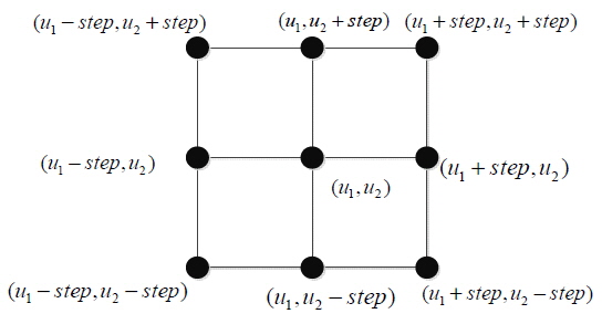
(2) Find an appropriate
(3) Select a new solution
(4) If the termination condition is satisfied, we have obtained the best solution; otherwise, go to step (2) and loop.
The flow chart is shown as Fig. 7.
2.6. Performance Metric of our FSO System
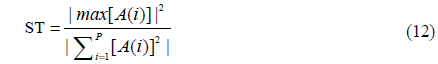
The goal of an adaptive optical system is to minimize residual phase aberrations after an incoming wave passes the deformable mirror. This corresponds to a maximization of the Strehl ratio (ST). In this paper, we use ST as the system performance metric

where

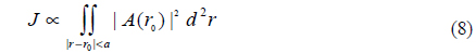
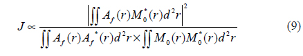
For direct optimization of the power coupled into a fiber, the system performance metric
Assume that the wavefront phase aberration satisfies a Gaussian distribution, ST can be estimated by variance RMS2 as follow

With increasing coupling efficiency, more energy is coupled into the single-mode fiber. When RMS2 is close to 0, we can get a simpler formula:

In practice, the pixel size of the CCD camera approximately equals the fiber diameter, so ST is [18]

where
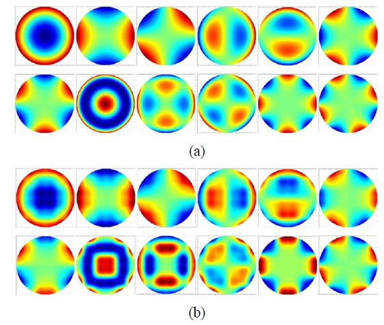
Based on the previous analysis, 12 Zernike modes and the corresponding correcting aberration are given in Fig. 8.
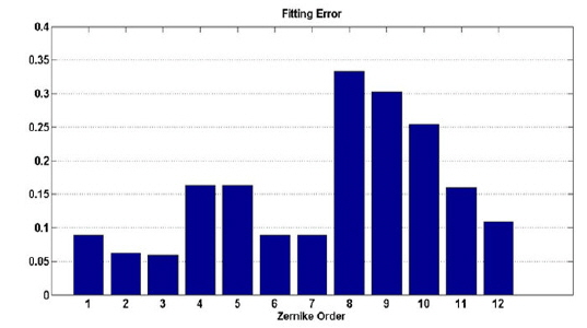
Define the fitting error as fitting capability for the wavefront aberration of DM [18]

where RMS
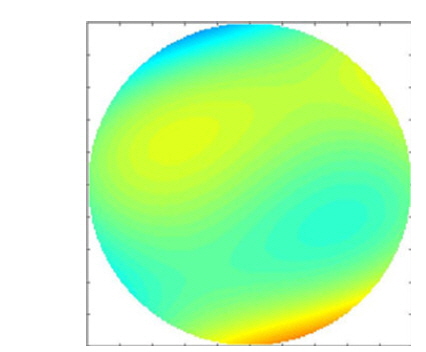
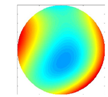
From Fig. 9 it is obvious that the DM has good fitting capability for the first 7 orders of wavefront aberrations. Generally, lower-order aberrations have the most important effect on intensity distribution and beam quality; therefore, we take only the first 7 orders into account. Note that a DM with higher spatial resolution and more actuators can accurately match more types of aberration modes. In our simulations, we introduce an incident wavefront with lower coupling efficiency (shown in Fig. 10).
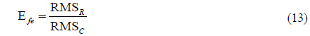
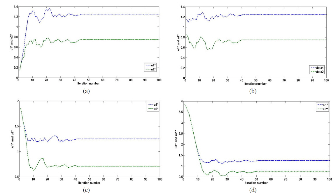
Our main target is to find the best solution group (
In Fig. 12, we compare the effects on this search process of starting with the different initial solutions (0, 0), (1, 1), (2, 2), and (4, 4) respectively. From Fig. 12 we find that different initial solutions lead to different search rates: The initial solution (4, 4) offers a faster search process (about 30 iterations), (2, 2) takes second place (35 iterations), and (1, 1) and (0, 0) do less well (about 40 iterations). The choice should be based on some practical experience and several tests.
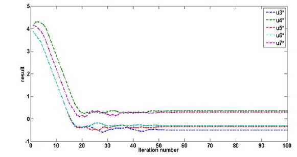
We also perform a fitting simulation of the remaining Zernike coefficients from
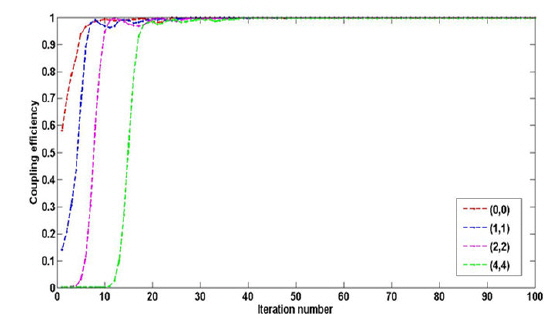
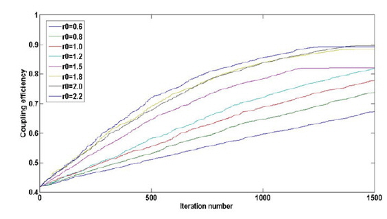
The variation of coupling efficiency with iteration number is shown in Fig. 15. We select the four different initial solutions mentioned above and find that the final coupling efficiency reaches about 99% in about 30 iterations.
We also perform some experiments to test the SPGD algorithm; the results before and after correction are shown in Figs. 16 and 17 [21]. In these experiments, we know that the MBTS algorithm is much faster than the conventional SPGD algorithm, usually requiring hundreds of iterations (Fig. 16), while the final coupling efficiency for both algorithms is similar. But the iteration number is largely inferior to that for MBTS even in theory, since the high-dimensional search space of SPGD reduces the searching rate, while in the MBTS algorithm we project a space with high dimension to a space with lower dimension and decouple them using a new system architecture. Thus the number of iterations will be sharply reduced, but only if the initial point is appropriately selected.
In Fig. 17, from the images received by CCD we see that the initial coupling efficiency before correction is very low, so that light scintillation is serious, but after correction the coupling efficiency is greatly improved. The corresponding results are in Table 1, and are inferior to the simulation results mainly because of the poor stability of the DM. This means that the DM should generate the identical corrected phase as by the same voltage applied to the actuators, in theory, but in practice it is limited by the skillful processing.
[TABLE 1.] Experimental results using SPGD
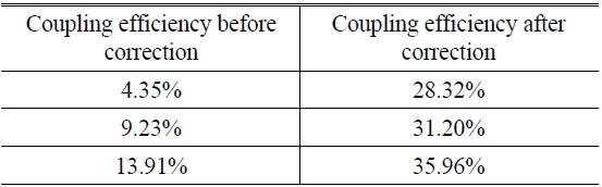
Experimental results using SPGD
We know that the singleshot correction assumption is a concern for the algorithm convergence speed and atmospheric coherenttime. The SPGD is a typical example in [13], with about 500 iterations in experiment, corresponding to 50 ms. The operation rate is limited by the MEMs DM (7-8 kHz) to satisfy the requirements of the AO system correction. Therefore, the corresponding convergence time of the MBTS is 5 ms to 6.25 ms with the new system model, but with some other algorithms (SPGD being the typical one), the time is tens of milliseconds. In the simulation, the time spent by the SPGD is about 90 ms when the coupling efficiency reaches 0.8; in our experiment, it takes 50-60 ms.
It is obvious that the SPGD works far less nicely than the MBTS. However, such a fast search (about 40 iterations) with the MBTS algorithm is at the cost of the construction of complicated equipment, with many sensorless AO subsystems working simultaneously. It places stringent demands on the experiment, and requires synchronization. This is the first such idea and system proposed in this research area, that many wavefront correctors may work in parallel to achieve better performance.
In this study we propose a novel algorithm, MBTS, to compensate the wavefront aberration from atmospheric turbulence in an FSO communication system based on a new parallel correcting system architecture. The new idea of the proposed algorithm and its results in an FSO system are described in detail. Simulations indicate that our proposed MBTS can offer a faster search process during optimization (dozens of iterations) and better final coupling efficiency, compared to the SPGD algorithm. The architecture of a novel and interesting parallel correcting system with multiple adaptive optical (AO) subsystems is also given.