Image deblurring by a deconvolution method requires accurate knowledge of the blur kernel. Existing point spread function (PSF) models in the literature corresponding to lens aberrations and defocus are either parameterized and spatially invariant or spatially varying but discretely defined. In this paper, a parameterized model is developed and presented for a PSF which is spatially varying due to lens aberrations and defocus in an imaging system. The model is established from the Seidel third-order aberration coefficient and the Hu moment. A skew normal Gauss model is selected for parameterized PSF geometry structure. The accuracy of the model is demonstrated with simulations and measurements for a defocused infrared camera and a single spherical lens digital camera. Compared with optical software Code V, the visual results of two optical systems validate our analysis and proposed method in size, shape and direction. Quantitative evaluation results reveal the excellent accuracy of the blur kernel model.
Many factors can contribute to the undesired blurriness of a photograph. While blur sources such as camera shake, subject motion and defocus have been studied well, and researchers have proposed effective solutions to restore the corresponding photos, degradations due to the camera optical system have received little attention. This is particularly inappropriate because optical degradations affect every photograph and cannot be easily removed. This problem is wellknown in the photography community as “soft corners” or “coma aberration”, and it is a discriminating factor between entry level lenses and professional-grade equipment.
When blur is undesirable, one can deblur an image using a deconvolution method, which requires accurate knowledge of the blur kernel. In applications where blur is desirable and essential, such as shape from defocus, it is still necessary to recover the shape and size of the spatially varying blur kernel. The point-spread function (PSF) is a quantization form of blur kernel, which describes how a point of light is redistributed over a local area of the sensor in an imaging system.
The key insight of our work is that a novel parameterized model will be developed and presented for a spatially varying PSF due to Seidel aberrations and defocus in an imaging system. A parameterized spatially varying model can provide a regularization mechanism, which constrains each individual blur estimate and constrains the relationship between neighboring blur estimates.
In this article, Section II describes related work on the spatially varying PSF model in other literature. Section III describes the estimation algorithm developed by Simpkins for the spatially varying PSF model constructed from Seidel aberrations and optical system parameters. [1, 7, 10, 13] The main contributions presented in this paper include comprehensive simulation of a proposed skew normal PSF model. Section IV and Section V presents results of a PSF model estimation experiment on a defocused infrared telescope system and a single lens digital camera with optical aberration. We compare the simulated results with standard PSF model generated from optical software Code V. Section VI presents conclusions and discusses the directions for future work.
Blur kernel models in the literature tend to fall into one of two categories: parameterized and spatially invariant or spatially varying and discretely defined. The downside of the spatially invariant model is that both simulation and experiments have demonstrated the need for PSF to have a spatial dependency. The downside of the discretely defined model is that it has many degrees of freedom for a PSF of reasonable size and requires a larger dataset for accurate kernel estimation. Additionally, there is no well-motivated mechanism to accurately interpolate the PSF for any particular point (x, y) in the image plane: other works on spatially varying blur have instead relied on ad-hoc interpolation of discretely defined PSFs corresponding to known points on the image plane.
Many techniques have been proposed to estimate and remove optical blur due to optical aberration, motion, and defocus. (See [1, 3, 4, 6, 7, 9, 10, 13, 14] and references therein.) Joshi et al. [3] estimate PSFs from edges in the image. They describe how to use a printed pattern to calibrate a camera at a given aperture and focal length and show that they can restore images taken later with the same parameters. The PSF can present spatially varying blur, which lacks a parameterized model. E. Kee et al. [6] introduce a method to estimate the blur kernel densely over the image and across multiple aperture and zoom settings. Simpkins and Stevenson [1, 7, 10, 13] have developed methods using geometrical optics to construct a parameterized model for a spatially varying PSF due to lens aberrations and defocus.
A similar approach based on Seidel aberrations and optical system parameters is selected in this paper. The major improvement brought by our work is that we use our measures to build a parametric model of the spatially-varying optical blur. Our results show that, with our model, PSF models are built for a defocused infrared telescope and for a single lens digital camera with optical aberration.
The Seidel aberration model describes the path of a single ray of light passing through a lens. A derivation will then be presented of a composite model, which will be used as the proposed ray tracing model to account for lens aberrations and defocus.
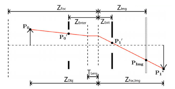
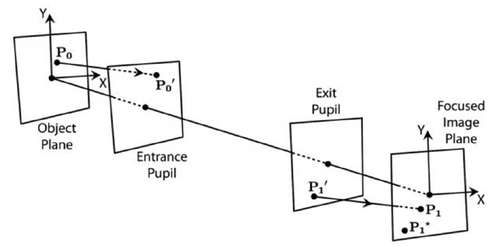
Figure 1 shows the Seidel aberrated ray tracing procedure. The Seidel aberration model describes where a ray leaving from a point P1’ on the exit pupil should arrive on the focused-image plane (at aberrated arrival point P1), given an ideal arrival point P1*. The model is based on a third-order Taylor series expansion of Snell’s law and assumes a spherical lens surface which is symmetric about the optical axis. A complete presentation of the Seidel model is given by Born and Wolf [2].
The Seidel aberration model requires only five parameters corresponding to the aberration coefficients representing spherical aberration (B), astigmatism (C), field curvature (D), radial distortion (E), and coma (F). [5]
The Seidel model describes the arrival point of the aberrated ray on the focused-image plane (the conjugate plane of the object plane), which is not necessarily the plane of the image sensor. In order to take defocus into account, the Gaussian thick-lens geometric optics model with offset apertures can be used to follow the path of a ray traveling from the object at point P0 to the image sensor at point PImg in Fig. 2. In this model, the lens is represented by a pair of equivalent refractive planes, which are separated along the optical axis by a distance TLens.
In the common case of a lens containing many optical elements, the thick-lens model with offset apertures is an approximation to the overall effect of the lens. Therefore TLens, ZEnter, and ZExit may be the effective thickness and offsets of the thick-lens approximation and not the actual lens thickness or the locations of the physical lens pupils [16, 20].
M is the magnification from entrance to exit pupils. Z1 and Z2 are the distances of the focused-image and the image planes, respectively, to the exit pupil of the system, and P1* is the nonaberrated arrival point of the ray on the focused image plane. These simplifying parameters are computed from the thick-lens model as Eq. (1) - (3), these parameters are the base of PSF model formation.


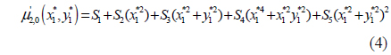
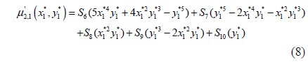
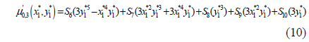
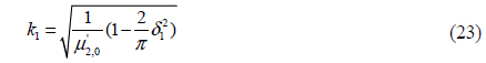
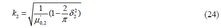
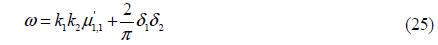
The Hu moment has a clear analogy to the moments of a joint bivariate probability distribution function. Following this analogy, the Hu moment is extended to the concept of a normalized central moment μ’pq. Calculating this integral for p, q∈{0; 1; 2; 3}, the normalized second- and third-order central moments can be solved as functions of the aberration coefficients, the aperture radius, the focus and object distances, and the location in the image plane [Eq. (4) - (10)].


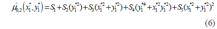
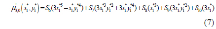

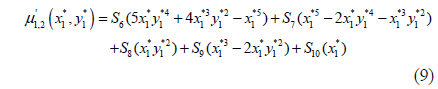

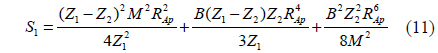
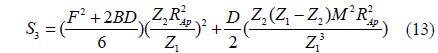
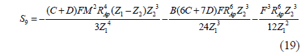
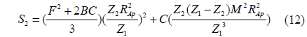
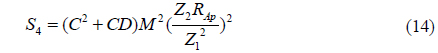
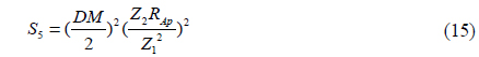
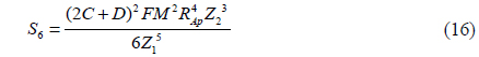
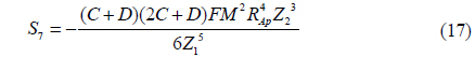
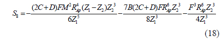
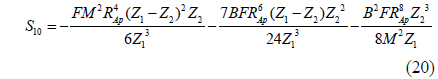
where the constants S1,…,S10 are introduced to make the central moments polynomial functions of the point P1*(x1*,y1*) across the focused image plane, and the constants are determined from the optical parameters of the camera as Eq. (11) - (20).


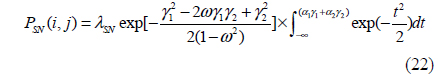
Because of the characteristic of the normalized central moment, the central moment and Seidel coefficients can be united in PSF model construction. The proposed model of S1 - S10 takes a set of predicted Hu moments and produces the corresponding estimate of the surface of the instantaneous PSF. There are two candidate models for the instantaneous PSF that will be evaluated in this article: the elliptical Gaussian model and the bivariate skew-normal distribution. The elliptical Gaussian model is specified entirely by the second-order central moments [8].
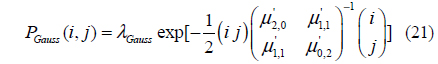
Unfortunately, the Gaussian PSF model cannot represent skew (it requires all four of the third-order moments to be zero). This is a major shortcoming of the Gaussian model, because with a lens that exhibits coma (represented by Seidel aberration coefficient “F”), the resulting lens-effect PSF can display significant skew. Interestingly, it is shown in Eq. (4) - (10) and (11) - (20) that if the coma coefficient F goes to zero, all third-order moments also go to zero, regardless of the values of the other four Seidel aberration coefficients. To allow for nonzero skew, we select the bivariate skew-normal distribution model shown in Eq. (22)

where


IV. DEFOCUSED INFRARED TELESCOPE
4.1. Results of Focused Infrared Telescope
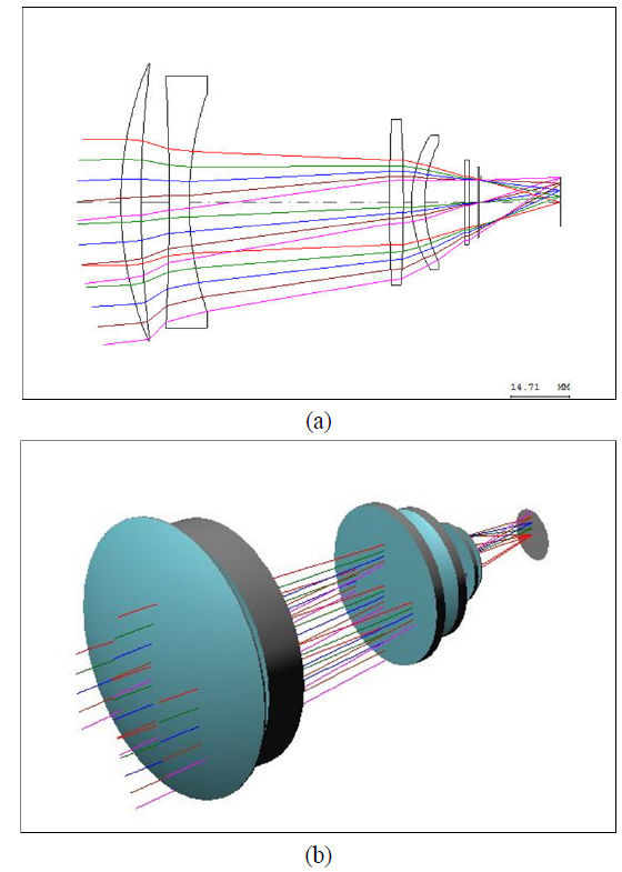
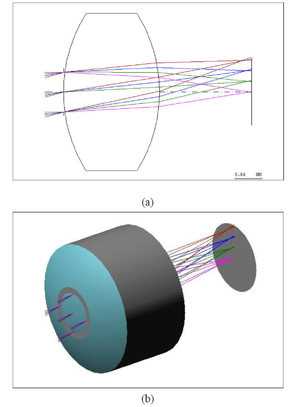
To test the proposed method, the PSF model is estimated with a real infrared telescope optical system. An infrared optical system with four spherical lenses is selected whose basic specification is listed in Table 1 [22-24]. There is no reflector in this camera, and every refracted surface figure is spherical. The glass material, silicon and zinc selenide are very common optical materials in an infrared telescope.
[TABLE 1.] Parameters of infrared telescope optical system
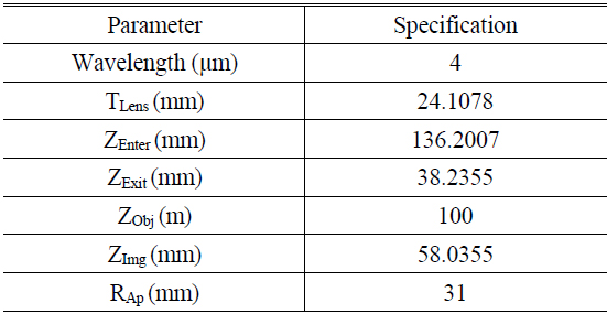
Parameters of infrared telescope optical system
Figure 3 shows the 2D ray tracing model and 3D construction of the infrared system.
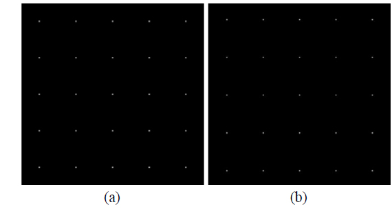
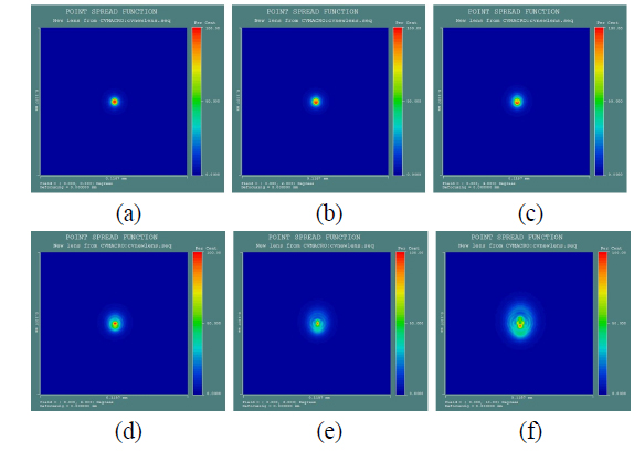
First, we estimate the PSF model from the focused infrared camera. The standard PSF model is generated by optical design software Code V, shown in Fig. 4. There is no optical blur in the focused situation. Visual results indicate that both of the blur kernels are very small without optical blur shape.
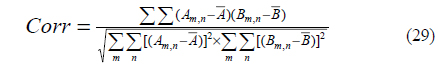
A correlation coefficient is used as a metric to evaluate the results of PSF models. Corr is the computation of the correlation coefficient of matrix A and matrix B. The computation algorithm of Corr is shown in Eq. (29).

where is the average value of matrix A, and similarly for parameter and matrix B. When the correlation coefficient value is close to 1, results indicate that there is a positive linear relationship between the two matrices [11].
Compared with the simulated PSF and standard PSF from Code V, Fig. 5 shows the correlation coefficient distribution with different field angles, and the average correlation coefficient is 0.8003.
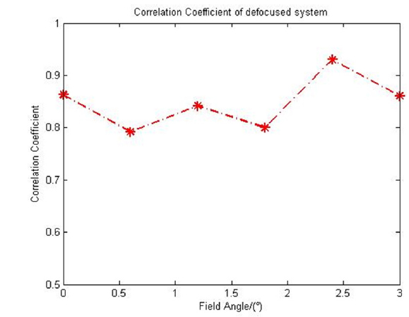
4.2. Results of Defocused Infrared Telescope
In this optical system, 0.2 mm defocused distance from perfect image plane is adjusted to estimate the PSF model in defocused condition. Results are shown in Fig. 6. There is symmetrical optical blur without coma component in any field angle.
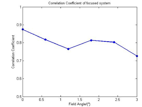
In defocused condition, comparing the simulated PSF and standard PSF, Fig. 7 shows the correlation coefficient distribution with different field angles, and the average correlation coefficient is 0.8479. All the correlation coefficients are higher than 0.75 in focused and defocused systems. Results show that this method can accurately estimate PSF in a defocused optical system.
V. SINGLE LENS CAMERA WITH OPTICAL ABERRATION
To test the optical aberration characteristic, a single lens optical system designed for digital camera or mobile phone camera is selected. To reduce the system length, there is only one single spherical lens in the optical system. However, correction of coma, astigmatism, field curvature, distortion and chromatic aberration must rely on stacking up additional lens elements. Spherical aberration can be avoidable by using an aspheric lens element. Because an imaging system using this lens can be manufactured massively at a very low cost, and its inherent defect produces very strong optical aberrations, it is a perfect optical system to test the spatially varying PSF model for optical aberration. Figure 8 shows the 2D ray tracing model and 3D construction of the one spherical lens optical system of the digital camera. All of the parameters of the single lens optical system are given in Table 2.
[TABLE 2.] Parameters of single lens camera optical system
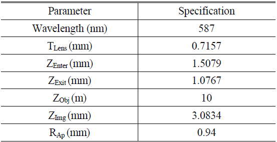
Parameters of single lens camera optical system
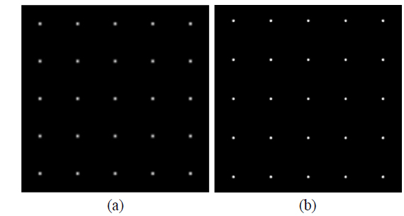
In Fig. 9, Cartesian PSFs model generated by Code V are segmented into several regions with different field angles 0° to 10°. PSF models in the Cartesian domain vary from region to region, not only in size, but also in shape and direction, resulting in a spatially variant distribution. Fig. 10 shows the shape and direction comparison of the simulated PSF surface with standard PSF from Code V.
In Fig. 9 and Fig. 10, diffraction phenomenon can be simulated from optical software Code V and Zemax. In classical physics, the diffraction phenomenon is described as the interference of waves according to the Huygens-Fresnel principle. In the proposed method, the PSF model is constructed from Seidel aberration coefficients based on the Taylor series of Snell’s law. The simulated PSF model cannot present diffraction phenomenon due to the difference of geometrical optics principles and physical optics principles.
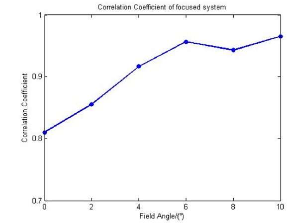
As mentioned above, the correlation coefficient is used as a metric to evaluate the results of aberration PSF. The average value is higher than 0.9, the distribution is shown in Fig. 11. As part IV proved, the correction coefficient of Fig. 11 goes higher as the field angle get larger, because the outer field is more defocused. The results show that the proposed model can provide good accuracy of the blur kernel model for optical aberration and for a defocused system.
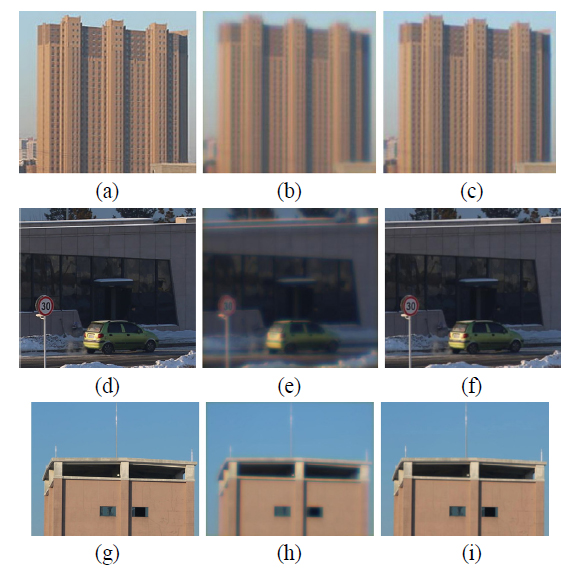
At last, in order to verify the truth of constructed PSF model, image restoration by different numbers of segmented regions was implemented. The blurred polar images were segmented into different numbers of locally invariant regions and restored by applying different numbers of polar PSFs [19]. The image restoration effects on an apartment building, car and observing tower are shown in Fig. 12, captured by 5D mark III with EF 100 mm f/2 USM.
Motivated from an established theoretical framework in physics, we conclude that the proposed spatially varying model is able to accurately describe the second- and third-order Hu moments of a set of spatially varying PSF across the image plane. The model has been validated by means of the simulation results of an optical system with defocus and optical aberration
There are two imperfect characteristics to the proposed method. First, when any essential parameter of the optical system is inaccurate, a big deviation error will probably appear in PSF model formation. Estimating blur kernel based on blur image can make up this deficiency and increase the robustness. Second, because of the difference of geometrical optics and physical optics, the simulated PSF model cannot present diffraction phenomenon. In the future we will try to integrate these two principles to provide a more accurate PSF model.