The geometrical theory of diffraction (GTD) [1] has played a prominent role in high-frequency analysis of electromagnetic scattering and diffraction. The asymptotic diffraction coefficients of a perfectly conducting wedge, which was rigorously derived more than one century ago, laid the foundation of the GTD technique. Until now, however, there have been no rigorous diffraction coefficients of penetrable wedges. As a detour, we performed the physical optics (PO) approximation on the lit boundary of a dielectric wedge [2]. Next, the correction to the PO diffraction coefficients was implemented by numerically calculating the non-uniform currents on its lit and shadow boundaries [3,4].

Recently, the finite difference time domain (FDTD) method has been employed to calculate the diffraction coefficients of penetrable wedges numerically without any analytical treatment [5]. However, the fully numerical approach could not provide any physical understanding of the inherent features in the wedge diffraction. On the other hand, a systematic tracing of the geometrical rays, which are reflected and refracted on the shadow boundary of a penetrable wedge, was presented. This technique, called the hidden rays of diffraction (HRD) [6], provided more accurate diffraction coefficients of some canonical penetrable wedges [7-9] than the conventional PO solutions. In this paper, the physical background and fundamental issues of the HRD technique are reviewed in detail by reinterpreting the diffraction coefficients of a perfectly conducting wedge.

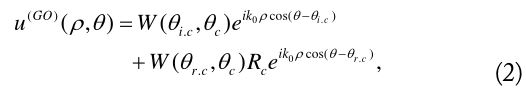
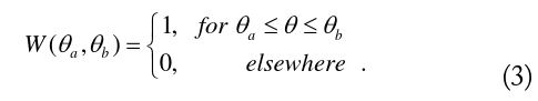
For a wedge illuminated by a plane wave, its geometrical optics (GO) field is expressed by a finite sum of ordinary rays, which are incident, reflected, and refracted on the lit boundary. Here the term ‘ray’ denotes a plane wave with the same amplitude and propagation angle. In contrast, its PO solution is given by an integral of the diffraction coefficients along the Sommerfeld’s path P [10]. The PO diffraction coefficients consist of the same number of cotangent functions as the ordinary rays. In asymptotic integration, the P path is deformed into the steepest decent path (SDP) [10] and the closed P-SDP path. Then the integrations of the PO diffraction coefficients along the contour P-SDP and the SDP are equal to the GO term and the edge-diffracted field, respectively. Therefore, there is oneto-one correspondence between the ordinary rays of its GO field and the diffraction coefficients of its PO field [2,6]. It causes the PO diffraction coefficients to be constructed routinely only from the conventional ray-tracing data.

In general, however, the PO field cannot satisfy the boundary condition at the wedge interface and the edge condition at the wedge tip. The GO field is the perfect first term of the asymptotic series solution in high frequency. The error of the PO field is then generated by the PO diffraction coefficients as the imperfect second term. From the traditional point of view, the error of the PO diffraction coefficients could be corrected by adding the non-uniform currents on wedge interfaces. In particular, both non-uniform currents on the lit and shadow boundaries are required for the same physical reason and are expressed in the same mathematical form.

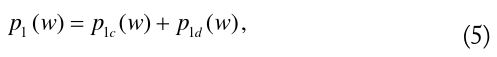
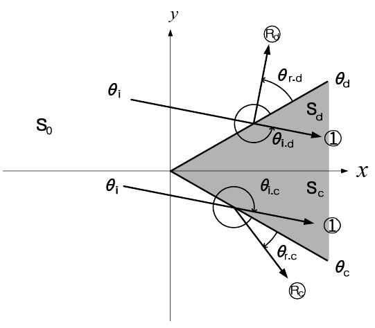
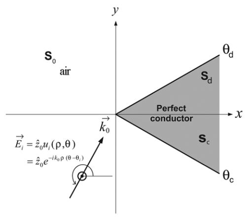
The starting line of the HRD technique was the comparison between the PO and exact diffraction coefficients of a perfectly conducting wedge. Consider an E-polarized plane wave incident only on its lit boundary at θ = θ_c, as shown in Fig. 1. In this case, the PO solution u^(PO)(ρ,θ) and exact total field u^(ex)(ρ,θ) were expressed in the same asymptotic integral form [10] as

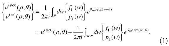
In Eq. (1), the GO field u^(GO)(ρ,θ) is well known as

where the angular window function W is defined by

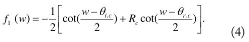
The PO diffraction coefficients f₁(w) are written by

The exact diffraction coefficients p₁(w) are given by

Where

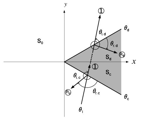
Each pole of the cotangent functions in Eqs. (4) and (6) denotes the propagation angle of the corresponding ray, as shown in Fig. 2. It should be noted that the propagation angle of a ray in Fig. 2 is accounted for by the sum of the angle of its reference line and the variation angle of its angular arrow. When the direction of the angular arrow is counterclockwise (clockwise), the variation angle is considered as a positive (negative) value. Both reflection amplitudes R_c and R_d are equal to -1 in this case.

Two cotangent functions in Eq. (6a) can be constructed from the PO diffraction coefficients in Eq. (4) only if the angular period of the cotangent functions is adjusted from 2π to 2πv_∞, where v_∞ is obtained from the edge condition [11] at the wedge tip as

Considering the one-to-one correspondence between the ordinary rays and the PO diffraction coefficients, one may routinely construct two cotangent functions in Eq. (6a) only from the ordinary ray-tracing data and the edge condition. This leads us to conclude that the ordinary rays on the lit boundary generate the first two cotangent functions in Eq. (5).

In Fig. 1, the incident field cannot reach the shadow boundary at θ = θ_d . Therefore, no actual reflection occurs on the shadow boundary. However, the exact solution in Eq. (5) consists of four cotangent functions, among which the last two should directly relate to the reflection on the shadow boundary. In a pure mathematical way, Fig. 2 illustrates the propagation angles and amplitudes of the incident and reflected rays on the θ = θ_d boundary. According to traditional optics, however, there is no systematic way to trace the geometrical rays on the shadow boundary. Therefore, it is impossible to see these rays in the physical region. Thus, these extraordinary rays are called hidden rays [5].

Several arguing points are posed vis-a-vis the so-called hidden rays. The first issue is how to infer the physical existence of the hidden rays on the shadow boundary from the mathematical expression in Eq. (6b). In case of Fig. 1, not only the lit boundary at θ = θ_c but also its edge as the end-point of the lit boundary are illuminated simultaneously by the incident plane wave. At first, the ordinary rays on the lit boundary provide the GO field. According to the GTD, the diffracted field in a wedge may be interpreted as the field radiated from the induced currents at its edge. The GO field at the edge as the end-point of the lit boundary then generates the corresponding edge-diffracted field, as shown in Eq. (6a).

Naturally, the incident wave in Fig. 1 cannot reach the shadow boundary at θ = θ_d . Thus, no ordinary rays on the shadow boundary cause the corresponding GO field to be zero. However, the edge as the end-point of the shadow boundary is illuminated by the incident plane wave. This implies that the edge-diffracted field radiated from the induced currents at the edge as the end-point of the shadow boundary cannot become zero, as shown in Eq. (6b). In a reverse sense, one may guess that the diffraction coefficients in Eq. (6b) are also constructed from the hidden rays one by one.

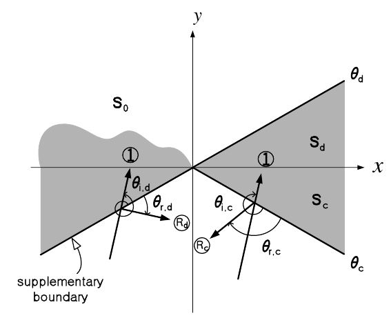
The above inference leads us to argue such the second issue as where the hidden rays exist. The poles of the two cotangent functions in Eq. (6b), which are directly equal to the propagation angles of the two hidden rays in Fig. 2, are well known as

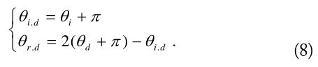
One cannot intuitively divine the physical meaning of the angles in Eq. (8). As a detour, consider that both boundaries of the wedge in Fig. 1 are illuminated by the incident plane wave for θ_d < θ_i < θ_c . The ordinary ray-tracing result in this case is shown in Fig. 3. It is an interesting feature that the propagation angles of two ordinary rays on the θ = θ_d boundary are also expressed by Eq. (8). In other words, hidden rays on a shadow boundary can be traced according to the same ray-tracing rule when the shadow boundary is illuminated by the plane wave with a different incident angle.

The third issue may be how to easily implement the visualization of the hidden ray tracing on the shadow boundary. As suggested in [6], a supplementary boundary was introduced by rotating the shadow boundary by 180° toward the air region. Then, as shown in Fig. 4, the incident plane wave can be incident on the supplementary boundary corresponding to the shadow boundary. It should be noted that the angle of the supplementary boundary is not θ_d + π but θ_d because its introduction is only for the visualization of the hidden ray tracing.

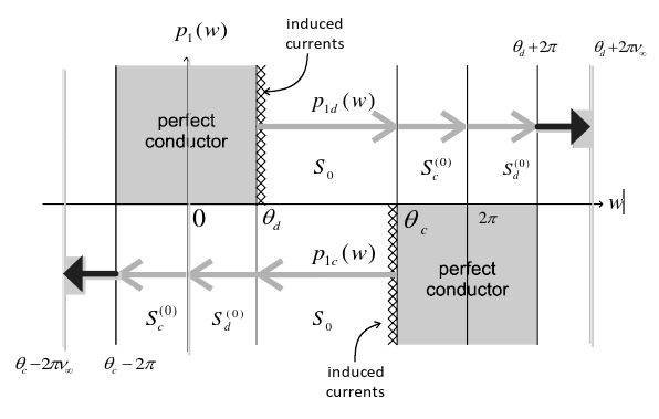
The last issue is strongly related to the angular period of the diffraction coefficients. The PO cotangent functions in Eq. (4) have the angular period 2π . In contrast, the angular period of the exact diffraction coefficients increases up to 2πv_∞ because according to Eq. (7), v_∞ is a positive real value larger than 1 but less than 2. The induced currents on the lit boundary then generate the diffraction coefficients p_1c(w) in Eq. (6a), as shown in Fig. 5. Because the angular period of p_1c(w) is 2πv_∞, its angular distribution range should be down to θ_c - 2πv_∞. On the other hand, the diffraction coefficients p_1d(w) generated from the induced currents on the shadow boundary should be distributed up to θ_c + 2πv_∞.

The physical air region S₀ in Fig. 1 is [θ_d, θ_c]. Based on the formulation of dual integral equations [2], the concept of the complementary air region was introduced [6]. The complementary air region S⁽⁰⁾_c is defined in the angular range of (θ_c, 2π] or (θ_c - 2π, 0] where the original conductor is replaced by air. In the same manner, S⁽⁰⁾_d denotes the other complementary air region in [0, θ_d) or [2π, θ_d + 2π). For convenience, the physical and complementary regions are limited to [0, 2π] . The exact diffraction coefficients are then expressed in different forms as

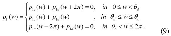
In particular, one may easily prove that the exact diffraction coefficients in two complementary air regions of [0, θ_d) and (θ_c, 2π] become zero, as shown in Eq. (9). This property is called the null-field condition in the complementary region.

This null-field condition has been used as a criterion to check the accuracy of the HRD solution to a wedge [6].

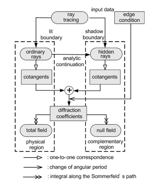
All the above properties formed a framework for implementing the HRD technique to solve a penetrable wedge problem. The standard procedure of the HRD technique, as illustrated well in Fig. 6, has provided more accurate diffraction coefficients of some canonical wedges [6-9].

In this paper, the physical existence and tracing rule of the hidden rays reflected and refracted on the shadow boundary are explained in detail by comparing the PO and the exact diffraction coefficients of a perfectly conducting wedge. The visualization of the hidden ray tracing on the shadow boundary is easily implemented by introducing its supplementary boundary. The null-field condition in the complementary region is also explained in detail. Compared to the physical theory of diffraction (PTD) [12], the HRD technique provides not only a pure analytic form of the diffraction coefficients of some canonical wedges but also a new aspect of the physical understanding of diffraction by a wedge. It is expected that this brief review will be helpful in applying the HRD technique to a wide range of diffraction problems.