It is important to know the substrate material parameters prior to designing an antenna, as the antenna figures of merit, such as the resonance frequency, bandwidth, efficiency, and physical size, are highly affected by its relative permittivity (εr) and loss tangent (tanδ).
Conventionally, the transmission-line (tx-line) method is often used to characterize material properties [1-3]. In this method, the scattering parameters (S-parameters) are firstly measured along with a microstrip line printed over the substrate. Then, the material parameters are extracted using closed-form equations derived from the fundamental tx-line theory. In these equations, εr and tanδ are expressed in terms of the S-parameters under the assumption of ideal transverse electromagnetic (TEM) wave mode propagation along the microstrip line. Thus, its accuracy can be significantly degraded by the higher order mode propagation. Furthermore, fabricating a separate txline can be regarded as a troublesome work if applications of the substrate under test are aimed for microstrip antennas.
In this paper, we present a material characterization technique that can measure the substrate εr and tanδ using an antenna as a test fixture, therefore, no additional tx-line structure is needed. Furthermore, instead of relying on restrictive closed-form equations, the material parameters are determined by comparing the measured reflection coefficient (S11) and bandwidth (BW) of the antenna to a set of full-wave simulation data. The latter is obtained by varying εr and tanδ in the simulation model. In the meanwhile, an optimization tool called surrogate-based optimization (SBO) [4-6] is employed to efficiently search for the global minimum of an error function formulated by the measured and simulation data.
In the following, effectiveness of the proposed method is verified by characterizing εr and tanδ of a substrate for a rectangular patch antenna. Section II presents the overall characterization process including the simulation model and error functions. Section III discusses test results based on full-wave simulations and Section IV demonstrates the validity of the method by measurements.
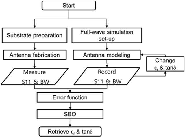
Changing εr and tanδ of the substrate affects the S11 and BW of the antenna. This leads to an inverse problem of determining εr and tanδ from those antenna figures of merit. With the higher εr, for instance, S11 at the antenna resonance frequency exhibits a sharper null due to the increase of stored energy inside the substrate (i.e., increase of the quality factor). On the other hand, the BW gets broader with the higher tanδ as more energy is dissipated inside the substrate. Fig. 1 shows the overall substrate characterization process. An antenna is fabricated on the substrate under interest, and then its S11 and BW are measured by a network analyzer. Concurrently, the same antenna is designed in a full-wave simulation tool, and a set of S11 and BW of the model is collected by varying εr and tanδ of the substrate. These simulated data are compared with the measured data in the error function via SBO technique. More specifically, we use the MATLAB Surrogate Modeling (SUMO) toolbox from Ghent University, Belgium [7]. This toolbox creates a kriging model of the error functions calculated from all sample points, and offers efficient algorithm to search for the εr and tanδ minimizing the error function. Finally, the retrieved εr and tanδ correspond to the substrate properties of the measured antenna.
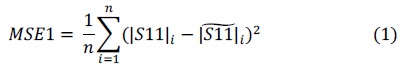
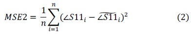
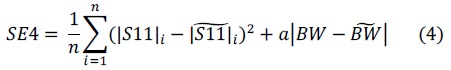
It is crucial to have a proper error function to secure accuracy and computational efficiency during the SBO process. Four error functions are tested in this study. All of them are combinations of S11 and BW in the form of mean squared error (MSE) as the following:
where |S11| and ∠S11 are the magnitude and phase of S11. The parameters with and without ‘~’ on the top correspond to simulation and measurement data, respectively. Also, n is the number of frequency points and a is a scaling factor. The latter is necessary for MSE4 calculation to keep balance between two different parameters, namely |S11| and BW. It is found that a = 20,000 guarantees the two parameters being in the same order, thus the optimization result is not more influenced by one of the parameters.
We note that using BW as one of the error function parameters is beneficial in collecting data compared to the antenna radiation efficiency often used in previous literatures [6]. For instance, the measurement of the radiation efficiency requires additional equipment set-ups, such as an anechoic chamber or Wheeler cap. On the other hand, BW can be conveniently measured by a network analyzer simultaneously with the S11.
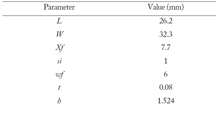
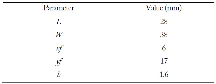
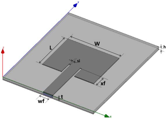
In order to validate the proposed method, a simulation study was performed by considering simulated data of a reference antenna as the measured data in the above mentioned process. Fig. 2 illustrates the geometry of the reference antenna model. An inset-fed microstrip patch antenna is designed to resonate at 3 GHz with the parameters given in Table 1. The conductive patch and ground are homogeneous copper foils with the conductivity of σ = 5.8 × 10⁷ S/m. The antenna substrate is the high frequency laminate RO4350B with εr = 3.66 and tanδ = 0.0031. These values are expected to be retrieved at the end of the process.
A set of antenna’s S11 and BW were collected using the same model but by varying εr and tanδ of the substrate. Eleven sampled points were assigned in the range of εr = (3.2, 4.2) and tanδ = (0.0001, 0.025), resulting in a total of 11 × 11 = 121 samples. For each sample, 101 numbers of S11 magnitude s and phase were collected throughout the test frequency range of f = (1.5, 3.5) GHz. Besides, BW was collected with |S11| < –6 dB criterion. It is worth noting that approximate values of εr and tanδ of the material under test is needed to set the data collection range. If the range is too broad or the sampling points are too sparse, it can be time consuming to collect data and compute the optimization result.
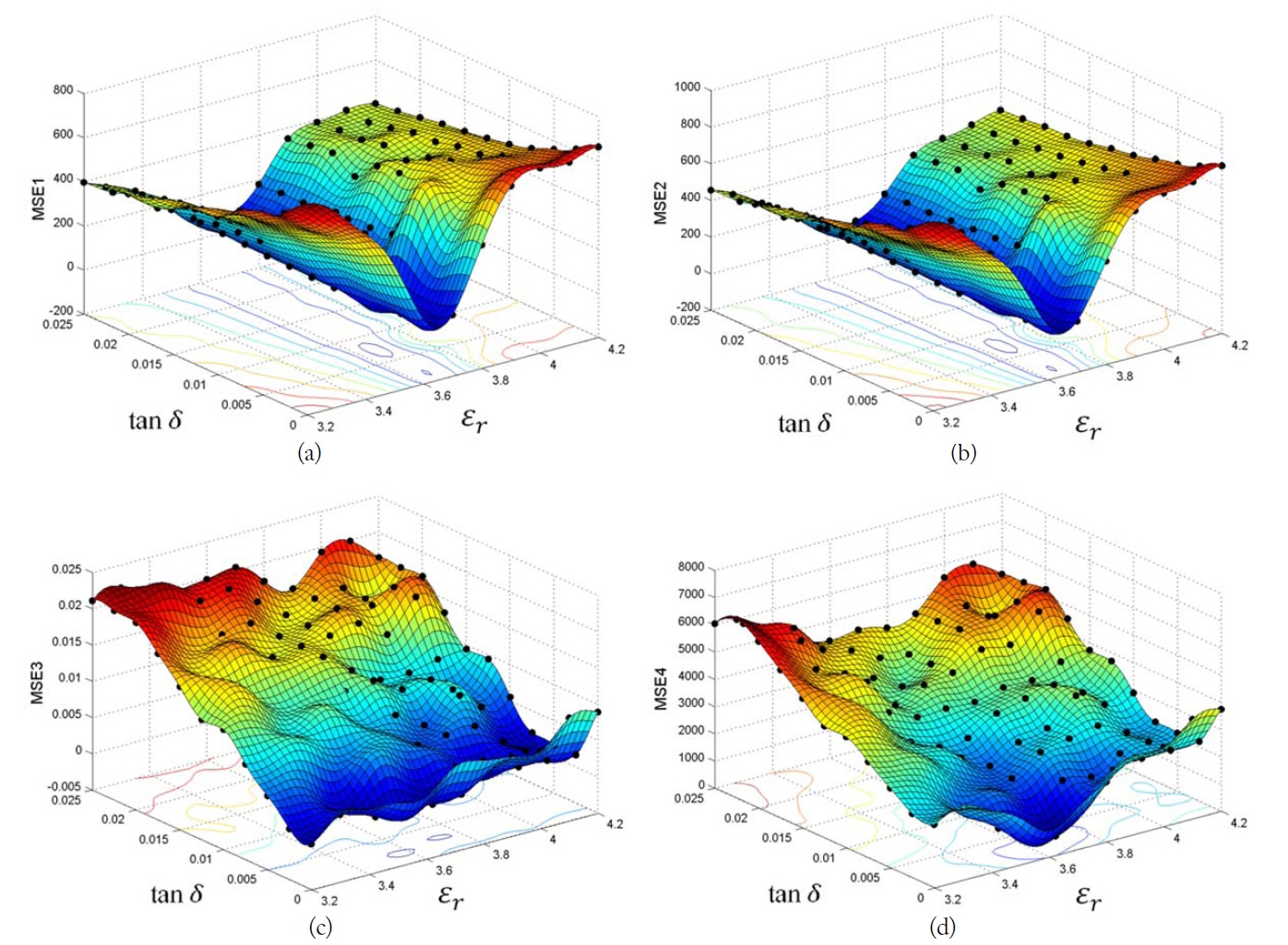
Fig. 3(a)–(d) show the optimization results (i.e. kringing models) after running the SBO process with the error function MSE1, 2, 3, and 4. It can be seen in Fig. 3(a) and (b) that the kriging models built from only |S11| and ∠S11 of the antenna have the similar distribution. They have a clear valley along with the εr -axis but not with the tanδ-axis. This implies |S11| and ∠S11 are suitable antenna figures of merit to evaluate the substrate’s εr. However, they are not appropriate to evaluate tanδ due to lack of sensitivity.
Fig. 3(c) shows the generated kriging model when only the BW is used in the error function (i.e. MSE3). Opposite to the previous, a clear valley is exhibited along with the tanδ-axis, meaning BW is more sensitive to the change in tanδ than εr.
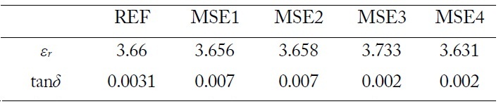
In regard to these observations, we can expect MSE4 formulated with both |S11| and BW is available to evaluate both εr and tanδ. This is verified in Fig. 3(d). As can be seen, the unique global optimum is located at the junction of εr = 3.631 and tanδ = 0.002 which are close to the given reference values εr = 3.66 and tanδ = 0.031. Table 2 summarizes the test results.
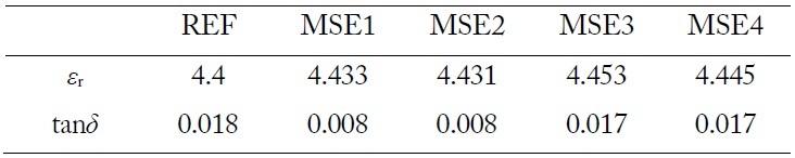
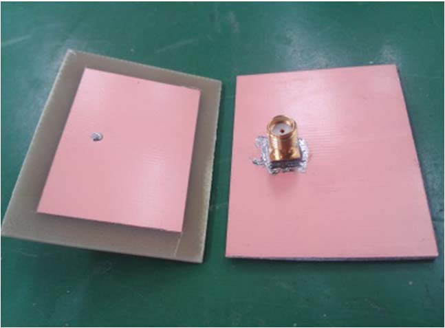
The proposed method is then validated with a patch antenna fabricated on a known substrate, FR-4. The material properties provided by the manufacturer of the substrate are εr = 4.4 and tanδ = 0.018. Fig. 4 is a picture of the fabricated antenna. It is fed by a coaxial probe and designed to resonate at 2.44 GHz. The antenna dimensions are given in Table 3.
The antenna’s S11 and BW are measured by a network analyzer (Anritsu MS2038C) and then compared to a set of simulation data using the same process described in the previous section. The test frequency range was f = (1.75, 3) GHz with the sampled interval of 10 MHz (i.e., n = 126 frequency points). The BW criterion was kept to be |S11| < –6 dB.
Table 4 presents a summary of the measurement results obtained from different error functions. Similar trends to the simulation results can be found. More specifically, MSE1 and MSE2 are more effective in measuring εr, while MSE3 has better accuracy in measuring tanδ. Finally, MSE4 yields the best result of εr = 4.445 and tanδ = 0.017, which offers a good agreement to the reference values from the substrate manufacturer.
In this paper, we reported an antenna substrate properties characterization technique. Measured and simulated responses of the antenna, S11 and BW, were collected, and then processed in the SBO algorithm with a proper error function. Four different error functions were evaluated. The results showed that the error function formulated by both S11 and BW was capable of retrieving the substrate εr and tanδ with high accuracy. Compared to the ordinary substrate characterization method, this method allows the use of an antenna itself as a test fixture. Also, the resulting data is highly accurate since the SBO algorithm together with full-wave simulation data offers solutions of complicated nonlinear problems, which are not considered in closed-form equations used in conventional methods. This characterization technique is inherently narrow-band since a resonating antenna is used as a test fixture. In this context, it is not suitable to retrieve the permittivity spectrum over a broadband.