The turbulent flow past a circular cylinder has been investigated extensively for a long time due to its importance in many engineering applications. It shows different features at different Reynolds numbers ( Re ), based on the free-stream velocity, cylinder diameter, and kinematic viscosity. There are three states of the flow with different Re : sub-critical ( Re =1000 ~ 2×10⁵ ), critical ( Re = 2×10⁵ ~ 3.5×10⁶ ), and super-critical ( Re > 3.5×10⁶ ) flows. In the sub-critical range the boundary layer along the cylinder is laminar and the transition to turbulence happens in the free shear layer downstream of the cylinder. With an increase of Re , the location of the transition moves upstream (Wissink and Rodi, 2008). In the critical range the base suction and drag decrease dramatically and this is associated with a revitalized boundary layer characterized by events in the order of a laminar separation, a transition to turbulence, a reattachment, and a turbulent separation further downstream with much reduced downstream wake width. In the super-critical regime, the boundary layer along the cylinder becomes turbulent before the separation. The base suction and drag of this regime is low due to the later separation of the turbulent boundary layer (Kravchenko and Moin, 2000).

The two-phase flow past an interface-piercing circular cylinder is much more complicated than the single-phase flow due to the interaction between the viscous effect near the body and the air-water interface phenomena, including wave run-up, breaking waves, thin liquid sheet formation, and air entrainment. It also exists in many engineering applications such as ship, ocean, coastal, and hydraulic engineering. The effects of the interface on the force distribution on the body, vortex generation and turbulence structures, and air-water interface structures, especially, their changes with the Reynolds and Froude ( Fr ) numbers are not well understood. A better understanding of these effects is also important for the cases when vortex- and/or wave-induced vibrations are to be considered.

There are several experimental and numerical studies on the flow past a surface-piercing circular cylinder in mainly subcritical Re regime. Inoue et al. (1993) conducted a towing tank experiment to investigate the characteristics of free surface turbulence for Re =27,000 and Fr =.8 and Re =29,000 and Fr = 1. They found that the periodic vortex shedding occurs in the deep flow, while this periodic vortex shedding is attenuated and higher frequency fluctuations are more prominent near the interface. Kawamura et al. (2002) investigated the wave-wake interaction about a surface-piercing circular cylinder using Large-Eddy Simulation (LES) based on a Smagorinsky Sub-Grid Scale (SGS) model at Re =27,000 with three different Fr =0.2, 0.5 and 0.8. At a low Fr , surface deformations were small and the influence on the wake was negligible. On the contrary, the generated surface wave was very steep and strongly unsteady at a high Fr . They also predicted significant surface fluctuations inside the recirculation zone immediately after the surface wave crest. In addition, they were able to visualize the attenuation of vortex shedding near the interface. Flows past an interface-piercing cylinder at various Re =1×10⁵ and up to Fr = 3 simulated using LES based on a Smagorinsky SGS model and a Volume of Fluid (VOF) method by Yu et al. (2008). They also showed that the free-surface attenuates the organized vortex shedding at the interface. At a higher Re, the free surface effect was reduced whereas this effect was enhanced at a higher Fr . As Re increases, the mean drag coefficient increases; however, it decreases along with Fr . They also showed that the dominant Strouhal number of the lift force decreased along with Re . Recently, Suh et al. (2011) studied the effect of air-water interface on the vortex shedding from a vertical circular cylinder for Re =27,000 and Fr =0.2, 0.8 using a high-fidelity orthogonal curvilinear grid solver. The organized periodic vortex shedding was observed in the deep flow whereas it was attenuated and replaced by small-scale vortices near the interface. The attenuation of the organized vortex shedding at the interface is caused by the streamwise vorticity and the outward transverse velocity generated near the edge of the separated region. The anisotropy between the vertical and transverse Reynolds normal stresses is the primary source of the streamwise vorticity and the outward transverse velocity near the interface.

The abovementioned studies were focused on relatively low Re and Fr in the sub-critical Re / Fr regimes ( Fr <1, sub-critical flow; Fr =1, critical flow; and Fr >1, super-critical flow). Chaplin and Teigen (2003) carried out an experimental study at higher Reynolds numbers up to 4.7×10⁵ and larger Froude numbers up to 1.67 with a constant Re / Fr ratio of 2.79×10⁵ . They found that the total resistance coefficient reached a maximum at Fr ~1. They also measured the run-up on the front of the cylinder and found that the run-up at a given Fr has a strong dependence on Re . However, their study was limited to resistance, run-up, and stagnation and base pressure measurements and analyses, many other flow features, such as the overall free surface and wave patterns, breaking waves near the cylinder, flow separation, vortex shedding, and other turbulent quantities, were not addressed. To the authors’ knowledge, this is the only recent study in the literature done on the turbulent flow past a vertical surface-piercing circular cylinder in the critical and super-critical Re / Fr regimes. As discussed above, the turbulent flow past a circular cylinder in the critical Re regime has very different flow physics than those in the sub-critical Re regime. Also the bow wave breaks in front of the cylinder for large Fr cases. Near the interface, the interactions of turbulence and interface are more complicated than the sub-critical Re / Fr cases studied in Suh et al. (2011) and the other work. Further investigations are required for better understanding of the effect of Reynolds and Froude numbers on the flow, especially, near the air-water interface.

To this end, LES of the two-phase turbulent flow past an interface-piercing circular cylinder at different Re / Fr with a constant ratio, same as Chaplin and Teigen (2003), are performed in the present study. This work can also be regarded as an extension of the precursory work for sub-critical Re and Fr (Suh et al., 2011). The same two-phase Navier-Stokes solver and computational domain, and similar grid sizes reported in Suh et al. (2011) are utilized here. In Suh et al. (2011), the Froude numbers were not high and there were no breaking waves. The level set method could effectively and accurately describe the evaluation of the air-water interface. However, for the super-critical Fr cases in this study, the level set method turns out to be too dissipative and incapable to capture the details of breaking waves. Therefore, a coupled level set and volume-of-fluid method (Wang et al., 2009; Wang et al., 2012) is employed to obtain a much improved interface capturing capability. In this study the effect of Re / Fr on the flow and the nature of unsteady free-surface are presented and discussed in detail. In addition, verification and validation of simulations are discussed using drag/friction/pressure coefficients, wave elevations, run-up height on the front face of the cylinder, and depression depth behind cylinder. Mean separation pattern, vorticity, Reynolds stress, and vorticity transport are studied for Re effects and air-water interface structures, vortical structures, and wave breaking phenolmena are investigated for Fr effects. Discussion is provided concerning the limitations of the current simulations and available experimental data along with future research.

CFDShip-Iowa version 6.2, a sharp interface orthogonal curvilinear grid solver for two-phase incompressible flows recently developed at IIHR (Yang and Stern, 2009; Suh et al., 2011) is used for all computations. The interface is tracked by a Coupled Level Set and Volume-of-Fluid (CLSVOF) method (Wang et al., 2009; Wang et al., 2012) instead of the level set method used in Suh et al. (2011) to capture detailed breaking waves.

An orthogonal curvilinear coordinate system is adopted for the governing equations. The Navier-Stokes equations for twophase, immiscible, incompressible flows have been written in the orthogonal curvilinear coordinates. The continuity equation is given as follows:

where u_i is the velocity in the orthogonal coordinate ξ direction and . J is the Jacobian of the coordinate transformation, defined as J = h_ih_jh_k , and with x_i a Cartesian coordinate.

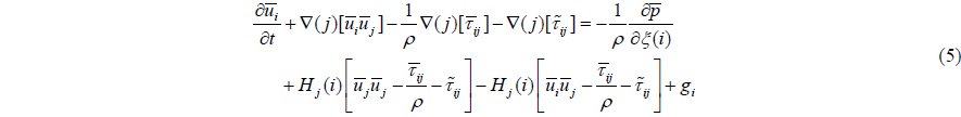
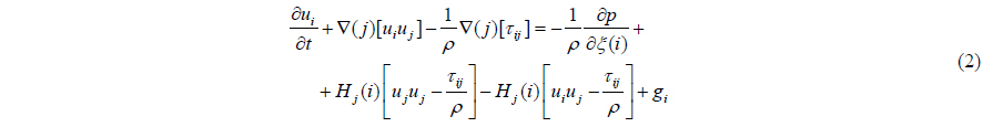
The momentum equations are given as follows:

where ρ is the density, p is the pressure, t is the time, and g_i the gravity vector in the ξ direction. Also, and ∂ξ(i) = h_i ∂ξ_i. The viscous stress tensor τ_ij is defined as follows:

where μ is the dynamic viscosity, ν_t is the turbulent eddy viscosity, and S_ij is the strain rate as defined as below:

In the LES approach adopted in this paper, the large, energy carrying eddies are resolved by spatial filtering of the governing equations whereas the small-scale, dissipative eddies are modeled by a SGS model. The Lagrangian dynamic SGS model based on Sarghini et al. (1999) is used in present LES. Eq. (2) is obtained as follows

with and , respectively. For simplicity, the filtering signs are dropped hereafter.

The interface is represented by the Level-Set (LS) function which is corrected using the VOF function to enforce mass conservation. The LS function φ is defined as a distance function which is negative in the air, positive in the liquid, and zero at the interface. The VOF function F is defined as the liquid volume fraction in a grid cell that gives zero in the air, one in the liquid, and a value between zero and one in an interfacial cell, respectively.

The LS function and the VOF function are advanced using following equations respectively.

Each phase of constant density and viscosity can be defined using the LS function in the computational domain and sharp jumps of the fluid properties occur at the phase interface. In this study, the density keeps its sharp jump and the viscosity is smoothed over a transition band across the interface (Yang and Stern, 2009).

The finite-difference method is used to discretize the Navier-Stokes equations on a non-uniform orthogonal curvilinear grid. A staggered variable arrangement is adopted, i.e., the contravariant velocity components u_i, u_j, u_k are defined at cell faces in the ξ_i, ξ_j , ξ_k directions, respectively, and all other variables are defined at cell centers. A semi-implicit time advancement scheme is used to integrate the momentum equations with the second-order Crank-Nicolson scheme for the diagonal viscous terms and the second-order Adams-Bashforth scheme for other terms. A fractional-step method is employed for velocitypressure coupling, in which a pressure Poisson equation is solved to enforce the continuity equation.

The convective terms are discretized using the non-conservative fifth-order Hamilton-Jacobi Weighted-ENO (HJ-WENO) (Jiang and Shu, 1996) scheme and all other terms are approximated using the second-order central difference scheme. A semicoarsening multigrid Poisson solver from the HYPRE library (Falgout et al., 2006) is used. Usually, the Poisson solver takes most of the computation time in a single time step.

The LS advection equation is solved using the third-order TVD Runge-Kutta scheme (Shu and Osher, 1988) for time advancement and the fifth-order HJ-WENO scheme for spatial discretization. To keep the LS function as a signed distance function, it has to be reinitialized after a certain time of evolution. The CLSVOF method (Wang et al., 2009; Wang et al., 2012) is used to re-distance the LS function and improve mass conservation properties of the LS method. In the CLSVOF method, the interface is reconstructed based on the VOF function with the interface normal computed from the LS function. The level set field is then re-distanced to reflect the position of the reconstructed interface, which satisfies the volume conservation constraint.

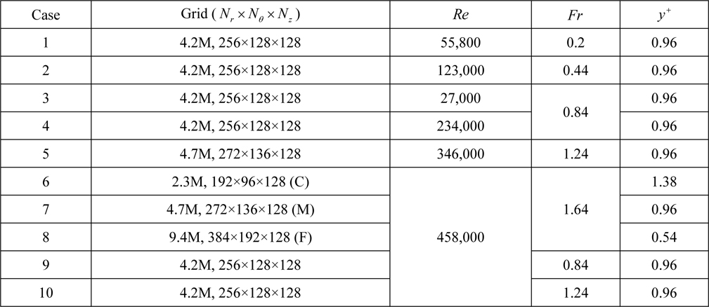
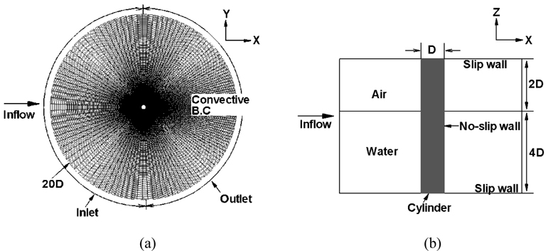
Body-fitted cylindrical grids were used for all cases and Table 1 shows the number of grid points and distance of the first grid point from the cylinder wall ( y⁺ ) for each case. Note that three different grids (coarse, medium, and fine) for Re = 458,000 and Fr =1.64 were used for a grid convergence study. The grid points are clustered near the cylinder wall to resolve the boundary layer and flow separation. Near the interface the grid was also refined to capture the interface deformation. Same as Suh et al. (2011), the computational domain was set up such that the portions of cylinder in the water and air are of length 4D and 2D with D the cylinder diameter, respectively. Note that this is the same aspect ratio used by Inoue et al. (1993), Kawamura et al. (2002) and Yu et al. (2008). The distance from the center of the cylinder to the outer boundary is 20D including a buffer zone to damp wave reflections as shown in Fig. 1.

The diameter of cylinder, D and the freestream velocity, U_∞ , were used for the normalization of all variables and the two non-dimensional parameters, Froude number and Reynolds number, are defined as follows:

As shown in Fig. 1(a), the outer boundary was divided into inflow and outflow boundaries at θ = 90° and θ = 270° , in which θ is the tangential angle starting from the downstream direction a nd a uniform inflow and a convective outflow boundary conditions were used. No-slip boundary conditions were applied on the cylinder wall, while the slip boundary condition was adopted at the bottom and the top of the computational domain as shown in Fig. 1(b). A uniform velocity field same as the upstream velocity is prescribed to the entire computational domain as the initial condition. In the present simulation, a constant Courant-Friedrichs-Lewy (CFL) number of 0.3 was used where the magnitude of the time step varied from 1×10⁻² to 1×10⁻⁴ D /U_∞ depending on the flow conditions.

The investigations cover 10 simulation cases, as also shown in Table 1. Cases 1-3 are for sub-critical and cases 4-10 are for post critical Re . Cases 1, 2, 4, 5 and 8 are for comparison with Chaplin and Teigen (2003). Cases 6-8 are for verification study at the highest Re and Fr condition. Cases 3, 4 and 9 are for Re = 27,000, 234,000 and 458,000 study at same Fr = 0.84 and Cases 7, 9, and 10 are for Fr = 0.84, 1.24 and 1.64 study at same Re = 458,000. Cases 1 and 3 are similar to Suh et al. (2011), but at a somewhat larger sub-critical Re and Fr, respectively.

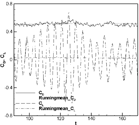
The time histories of the drag coefficient C_D and lift coefficient C_L with the running mean of C_D and C_L are shown in Fig. 2. The drag and lift coefficients are defined as

It should be noted that the still water depth, i.e., H = 4D here, and the water density are used for these coefficients (Kawamura et al., 2002; Yu et al., 2008; Suh et al., 2011). The statistically stationary state is defined using the convergence of the running mean from the time history of C_D . When the fluctuations of the running mean are smaller than 1% of the mean value, the flow is considered statistically stationary. After the flow reached steady state, 16 vortex shedding cycles, 80 non-dimensional time units, were used for statistics as shown Fig. 2.

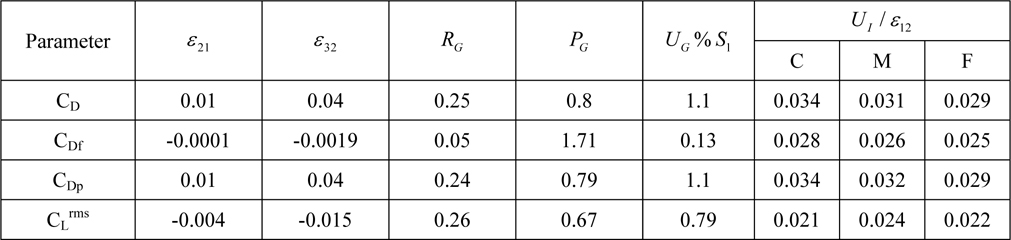
The grid verification study is performed following the methodology and procedures proposed by Stern et al. (2006) and Xing and Stern (2010) with three different grids (coarse, medium, and fine) for Re = 458,000 and Fr = 1.64 using four parameters (total drag coefficient C_D , friction drag coefficient C_Df , pressure drag coefficient C_Dp , and rms of lift coefficient C_L^rms). Verification is a process for assessing the simulation numerical uncertainty U_SN, defined as followed, U_SN² =U_I²+U_T²+U_G², where U_I is the iterative uncertainty, U_T is the time-step uncertainty, and U_G is the grid uncertainty. It should be noted that U_T was not considered in the present study due to the use of a constant CFL number, i.e. varied time steps.

Iterative convergence is assessed by examining the iterative history of drag forces and the iterative uncertainty U_I is estimated as half the range of the maximum and minimum values as shown below;

where S_U is the maximum solution and S_L is the minimum solution. In Table 2, U_I / ε₁₂ for three different grids are shown and its magnitude is one order smaller than that of the grid error.

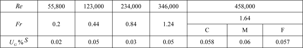
For all three grids, the iteration uncertainties are considered to be negligible in comparison to the grid uncertainties. Table 3 shows the iterative uncertainties for all the cases and it is less than 1% of the mean value of S , which also implies that the simulations are not contaminated by the iterative errors. so that simulation numerical uncertainty .

In Table 2, all the parameters show monotonic convergence using the grid refinement ratio r_G = 1.41 and the order of accuracy p_G for C_D, C_Df, C_Dp, and C_L^rms is 1.13, 1.71, 1.14, and 0.67 respectively and the grid uncertainty U_G for C_D ,C_Df , C_Dp , and C_L^rms is 1.1% S₁ , 0.13% S₁ , 1.1% S₁ , and 0.79% S₁, respectively.

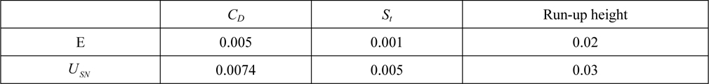
Validation is a process for assessing the simulation modeling uncertainty by comparing with experimental data D . The comparison error E is defined as the difference between D and the simulation S . If the absolute value of E is less than the validation uncertainty U_V , given by U_V² =U_D²+U_SN², where U_D is the uncertainty in the data, the combination of the all the errors in D and S is smaller than U_V and validation is achieved at the U_V level. As presented in Table 4, U_V of all the variables is greater than E although U_D is not available, which shows the present simulation has achieved the U_V level of validation.

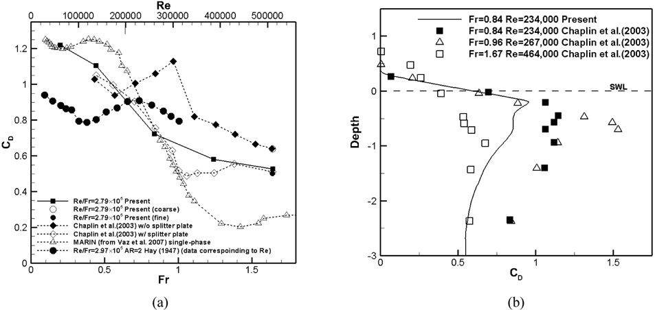
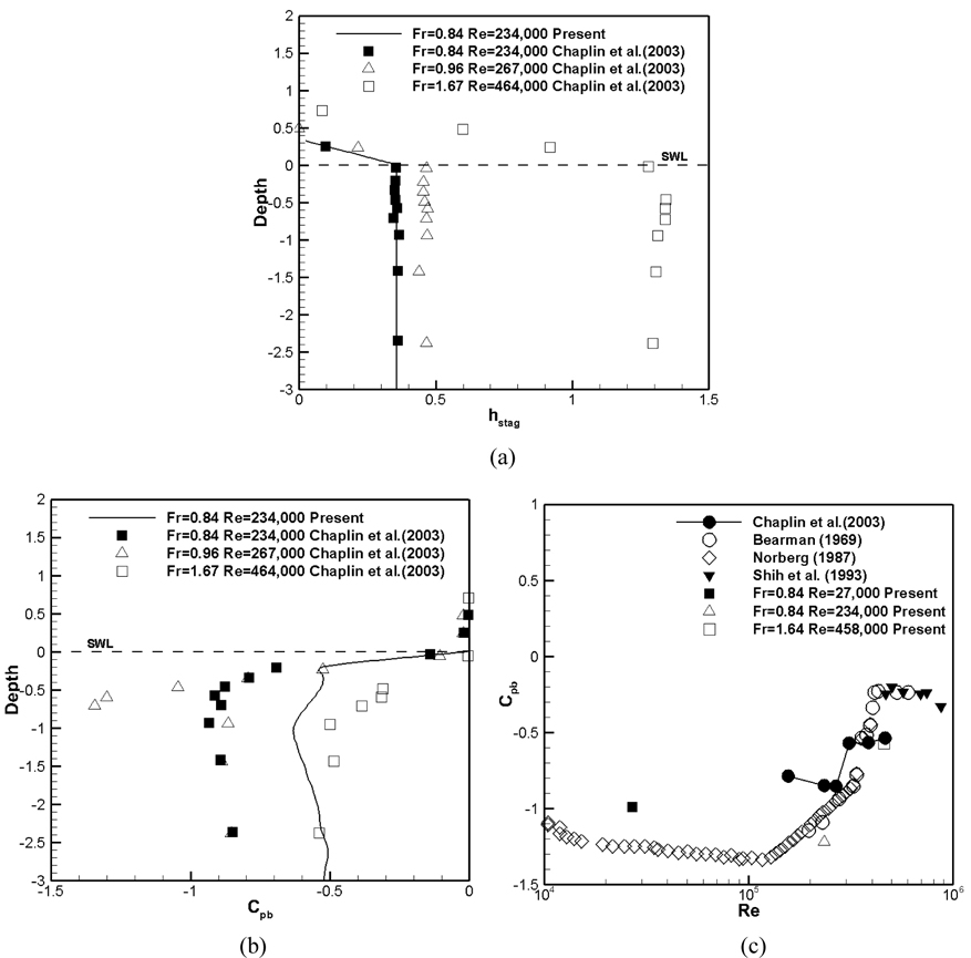
Fig. 3(a) compares present simulations with available experimental data for single and two-phase flow. All data is graphed for the correct Re scale; however, the single-phase data has no Fr correspondence and Hay (1947) two-phase data has a somewhat different Re / Fr = 2.97×10⁵ , whereas the present simulations and Chaplin and Teigen (2003) results are for Re / Fr = 2.97×10⁵ , as per both Re and Fr scales. Chaplin and Teigen (2003) experiments are for with and without splitter plate to suppress free surface effects, with end plate, for variable aspect ratio from 4-7, and subject free surface effects for Fr >.5 and blockage for all Fr. Hay (1947) experiments are for no end plate and aspect ratio 2 and also subject free surface effects. Note that the present simulations are subject free surface effects and for aspect ratio 4. As will be discussed later, for sub-critical Re aspect ratio needs to be larger than all current values to achieve single-phase benchmark conditions for the deep condition. The Chaplin and Teigen (2003) data with splitter plate is substantially smaller/larger than single-phase benchmark data for sub and post-critical Re, but with similar critical Re values. Chaplin and Teigen (2003) data without splitter plate and Hay have similar Re / Fr but different aspect ratio and experimental setup nonetheless somewhat similar trends: both show C_D max at critical Re and Fr near one (Fr = .75 vs. Fr = .96, respectively) and Hay (1947) has overall smaller values. Present simulations agree Chaplin and Teigen (2003) for sub and post critical Re but do not show increased values for critical Re and near Fr = 1. Fig. 3(b) compares present simulations with Chaplin and Teigen (2003) data without splitter plate for C_D vs. depth. Experiments show bulge in C_D below free surface for all Fr with maximum bulge for Fr=0.96. Simulations for Fr=0.84 show similar trends experiments for Fr = 0.84, but under predict C_D values.

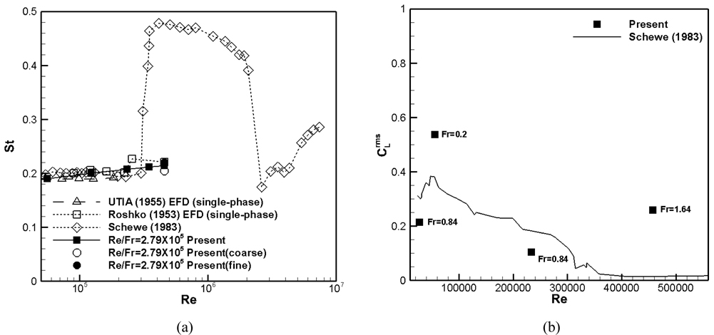
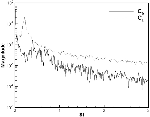
Fig. 4 shows the Fast Fourier Transform (FFT) of the C_D and C_L for Re = 458,000 and Fr = 1.64. The dominant Strouhal number ( St ) for C_L is obvious while the FFT of C_L shows a large range of frequencies. Fig. 5(a) presents St with different Re and Fr , including single-phase reference data. The results have good agreement with single-phase data for lower Re and the dominant St of the C_L increases with Re (and Fr ) increase, but not as much as one of the reference data. The dominant St from three different grids for Fr =1.64 are also shown in Fig. 5 and the fine grid simulation predicts closest with one of the experiments. Fig 5(b) shows CL RMS vs. Re , including single-phase reference data. The simulation trends for Fr = .84 are similar with the single-phase data in showing decreasing CL RMS with increasing Re . The simulations for Fr =.2 and sub-critcal Re show larger values than those for Fr =.84 and sub-critical Re . The simulations for post critical Re and Fr = 1.64 show larger values than single-phase data for same Re . Note that the present C_D , St and C_L RMS results for Fr = .84 and Re = 234,000 have close values to Suh et al. (2011) results for Fr = .8 and Re = 27,000.

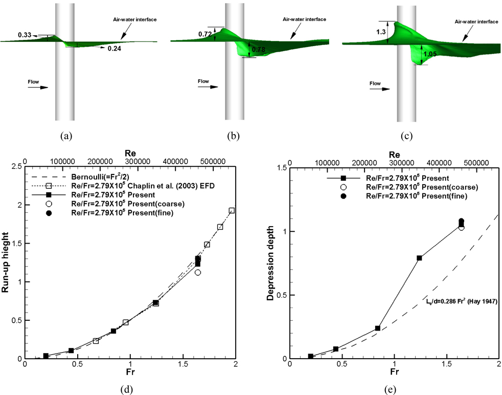
Fig. 6 shows the run-up height and depression depth with different Re and Fr numbers. The run-up height is the maximum bow wave height in front of the cylinder and the depression depth is the largest cavity depth behind the cylinder. Both run-up height and depression depth increase as Fr increases. The run-up heights of the present simulations have good agreement with the Bernoulli’s equation ( Fr² / 2 ) and the results from the previous study by Chaplin and Teigen (2003). Fig. 6 also shows the run-up height from three grids for Re = 458,000 and Fr = 1.64 and the fine grid has the closest to that from the Bernoulli’s equation and previous experiments (Chaplin and Teigen, 2003). The present results for depression depth agree with Hay (1947) for sub-critical Fr , but have larger values for super-critical Fr . A ratio between run-up height and depression depth for Fr = 0.84, 1.24, and 1.64 is 1.375, 0.97, and 1.23, respectively.

Flow field validation for Re = 234,000/ Fr = 0.84

In this section, the flow near the interface is compared with previous studies (Suh et al., 2011; Kawamura et al., 2002; Yu et al., 2008; Inoue et al., 1993). Note that the present simulation and the previous work have similar Fr , but different mostly subcritical Re .

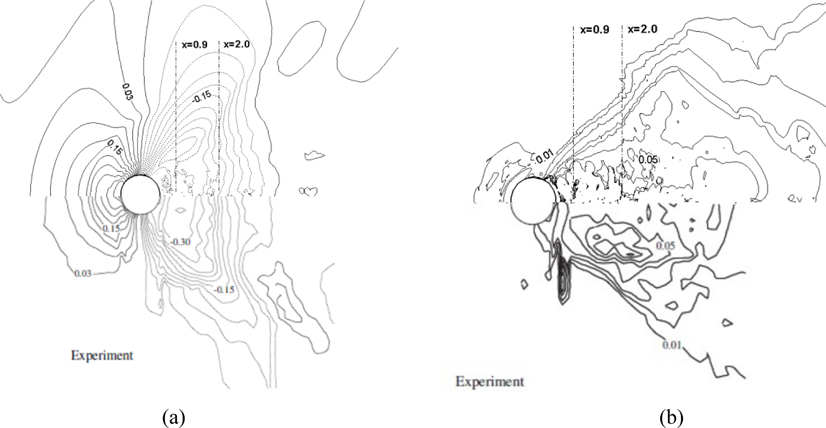
Contours of the mean interface elevation and the rms of the interface fluctuations are shown in Fig. 7 and compared with measurements by Inoue et al. (1993) using Re = 27,000 and Fr = 0.80. Overall, the present results of the mean interface elevation are in good agreement with the previous study (Inoue et al., 1993) including the magnitude, location of interface waves, and the expansion angle of Kelvin wave, although lower interface elevations are observed near the rear parts of the cylinder. The rms of the interface fluctuations from the current simulation also shows a good agreement with the experimental work (Inoue et al., 1993) including the location of the peak fluctuations.

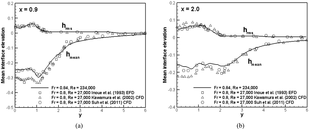
Fig. 8 presents the mean interface elevation and the rms of the interface fluctuations at two transverse planes for Fr = 0.84, comparing with previous studies (Kawamura et al., 2002; Suh et al., 2011) with Re = 27,000 and Fr = 0.8. The results of the current simulation with larger Re (= 234,000) are in good agreement with previous studies except for the under-prediction of the depression, which is also reported in Suh et al. (2011). In addition, this indicates that Re has little effect to the mean interface elevation behind the cylinder for sub-critical Re .

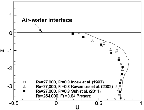
Fig. 9 shows the vertical profiles of the mean streamwise velocity at x = 4.5 and y = 0 for Fr = 0.84. The previous studies from Inoue et al. (1993), Kawamura et al. (2002), and Suh et al. (2011) of Re = 2.7×10⁴ and Fr = 0.8 were compared. Note that the fine grid solutions were compared for Suh et al. (2011). The present results for Fr = 0.84 agree with ones from Inoue et al. (1993), Kawamura et al. (2002), and Suh et al. (2011) near the air-water interface and it is clearly shown that the mean streamwise velocity decreases as the interface approaches. However, larger streamwise velocity profile is shown than previous studies in the deep flow.

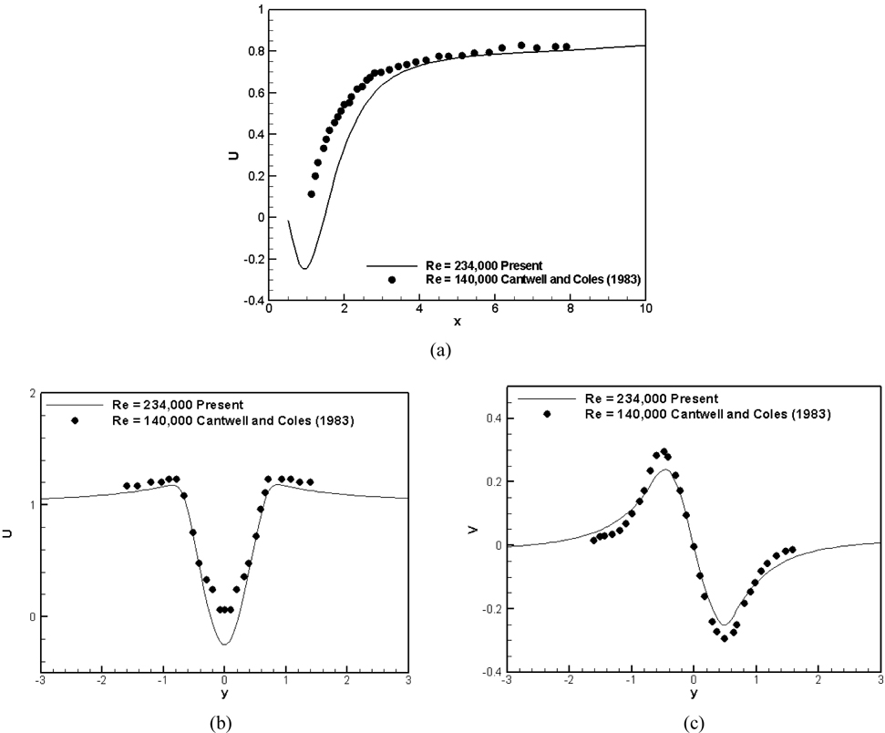
In this section, the flow in the deep water was compared with previous experiments on the single-phase flow past a cylinder at a similar Reynolds numbers as the present Re (=234,000) which is in the lower critical Re regime (Achenbach, 1968). Fig. 10(a) shows the mean streamwise velocity on the centerline at y = 0.0 along with the single-phase experimental measurements (Cantwell and Coles, 1983). Overall, the profile of the present simulation has a good agreement with the experimental data. The recirculation region is shown immediately after the cylinder ( x = 0.5 to x = 1.4) in the present simulation.

Fig. 10(b) and (c) shows the mean streamwise and transverse velocity in the wake at x = 1. For comparison the data of the experiments at Re = 140,000 (Cantwell and Coles, 1983) are also used. They agree fairly well with experimental data; however, larger streamwise velocity is observed and smaller transverse velocity is shown at y = 0.5 and y = -0.5.

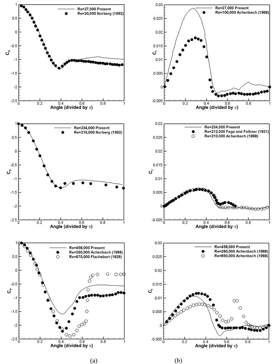
Fig. 11 presents the pressure and friction coefficients, defined as follows:

where τ_w is the wall shear stress. Some experimental measurements of the surface pressure and friction coefficients at close Re in single phase flows are also plotted for comparison and reference. For sub-critical Re , both the pressure distributions and skin frictions in the deep flow have a good agreement with the experiments. However, for post-critical Re , the predicted surface pressure still exhibits a sub-critical behavior, e.g., at Re = 458,000. Issues that may explain this behavior will be discussed later. Note that Suh et al. (2011) showed similar comparisons as Figs. 10 and 11 (for sub-critical Re ) for Fr = .8 and Re = 27,000 with very similar values.

Fig 12(a), (b) and (c) compares present simulations with Chaplin and Teigen (2003) experiments without splitter plate for stagnation pressure, base pressure coefficient vs. depth and in deep water vs. Re , respectively. The latter case includes benchmark single-phase data. Stagnation pressure increases with Fr similarly as run-up height with close agreement simulations and experiments. The experimental base pressure vs. depth shows similar trend as C_D vs. depth. The simulation for Fr =.84 is similar in shape to the experiments but under predicts the pressure magnitude. The experimental deep-water base pressure vs. depth shows large differences benchmark single-phase data. The present simulations for sub-critical Fr show smaller values than the experiments, whereas the values for post-critical Re agree with the experiments. Another issue with the experiments of Chaplin and Teigen (2003) is that their pressure measurements showed no clear evidence of vortex shedding for all cases.

Current results for sub-critical Re with fixed sub-critical Fr show similar trends with Suh et al. (2011) on run-up height, depression depth, mean surface elevation, and mean streamwise velocity. The drag coefficient in deep water is different with that of Suh et al. (2011) due to the difference in Re . Overall conclusion is that variation in sub-critical Re has small influence for fixed sub-critical Fr .

Three different Reynolds numbers from sub-critical to post-critical (27,000, 234,000, and 458,000) with Fr = 0.84 are used to investigate Reynolds number effect on flow structures near the interface.

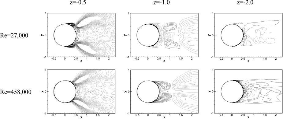
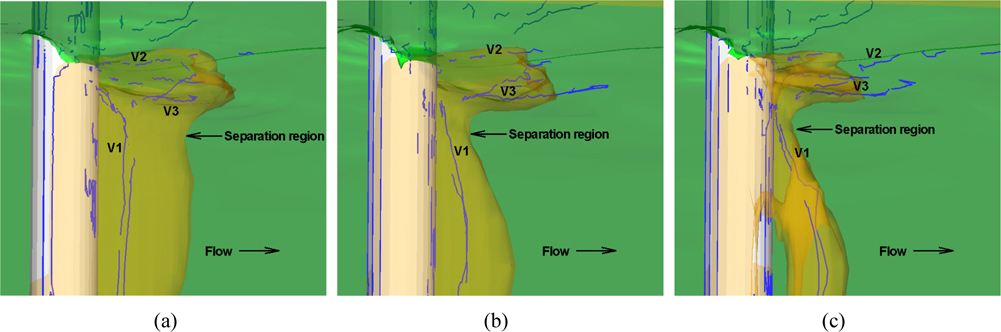
Fig. 13 shows the separation pattern of the mean flow with vortex core lines, which is obtained using the approach discussed in Kandasamy et al. (2009) and Sujudi and Haimes (1995). The separated shear layer was visualized approximately using the iso-surfaces of the stagnation C_p near the interface immediately before separation, assuming that the flow outside the separation is inviscid. Inside the separated region, the mean vortex core lines are extracted using the vortex core identifycation technique. The separated region at the interface decreases as Re increases from sub-critical to critical since the separation point is delayed, which is also shown in single-phase flow past a circular cylinder (Achenbach, 1968). Immediately below the interface, the separation region is reduced for all Re and “neck” shape is observed. The neck becomes narrower as Re increases. Three different types of vortices (V1, V2, and V3) were defined in Suh et al. (2011) as the mean vertical vortices, the mean streamwise vortices, and the V-shaped mean vortices and these vortices are observed in all Re . The vertical vortices (V1) are generated from the vortex shedding behind the cylinder and these vortices are inclined and connected to the cylinder wall as the interface is approached. The other two vortices (V2, V3) are observed inside the separation region near the interface as discussed in Suh et al. (2011). It is interesting to note the close resemblance between the mean separation pattern and the profile of the sectional drag coeffcient as a function of depth in Fig. 3(b); however, in present case for fixed Fr . Note that the present results for Re =27,00 are very similar Suh et al. (2011) for Fr = .8.

Vorticity

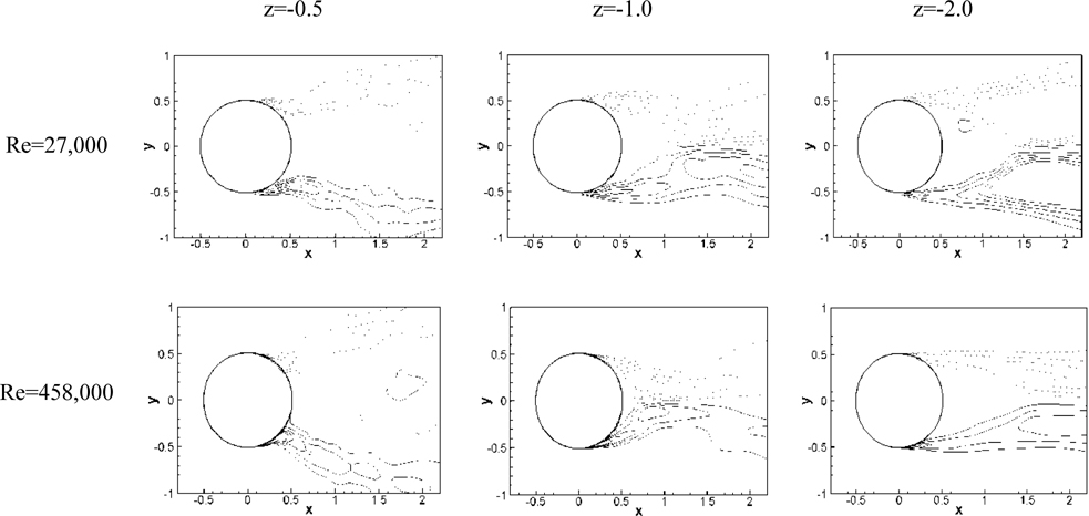
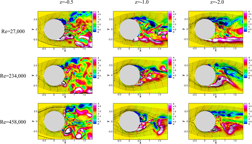
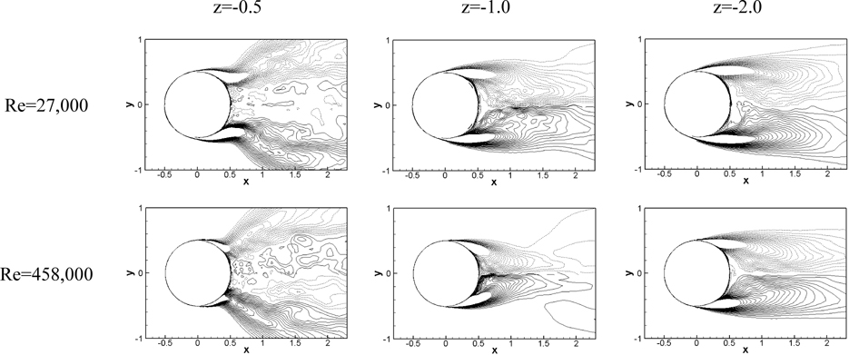
For a single-phase flow past a circular cylinder, the regular Karman vortex street and organized wake patterns are prominent for low Re whereas the separated shear layer becomes unstable and smaller vortices are generated at higher Re . Fig. 14 shows the instantaneous vertical vorticity contours with streamlines at various depths and different Re . Near the interface at z =-0.5 the attenuated vortex shedding. i.e., no organized periodic vortex is observed for all Re due to the streamwise vorticity generated near the separated region. However, the separation point is much delayed with an increase in Re . Suh et al. (2011) also showed that the delayed separation occurs near the interface. At z = -1 where the “neck” shape is formed, the narrowing of the wake is observed for the critical and post-critical Re (234,000, 458,000). In addition, the separation point moves downstream as Re increases. The narrow wake region becomes wider from z = -1 to z = -2 which is correlated to the recovery of the separation region as shown in the mean separation patterns.

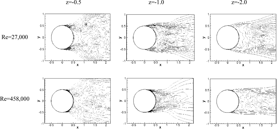
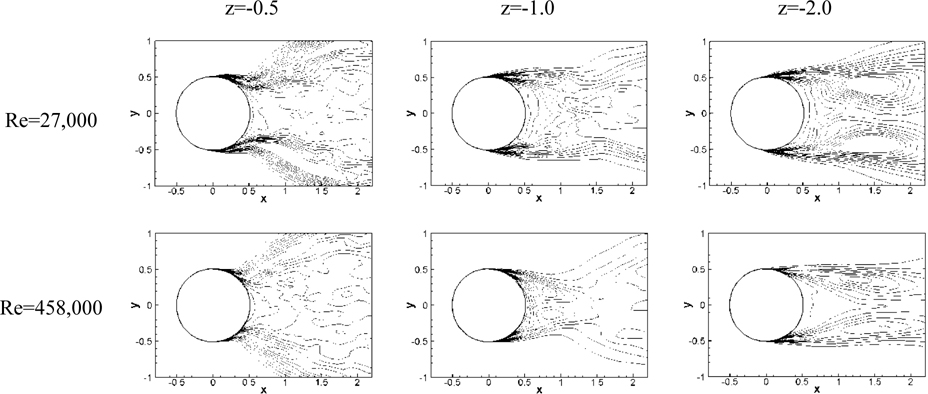
Fig. 15 shows the mean streamwise vorticity contours for two Re at three different depths. Near the interface small vortices are dominant instead of the organized vortices and more small vortical structures are observed as Re increases. In addition, the width of wake is significantly large for all Re . The maximum streamwise vortices are observed in the edge of the separation region. As discussed in Suh et al. (2011), three pairs of counter-rotating vortices are observed at z =-1 for Re =27,000 while only two pairs of counter-rotating vortices are shown with much reduced wake region for critical Re due to the delayed separation point and smaller recirculation region. The increased wake region and strong transverse velocity near the interface are generated from these vorticity pairs (Suh et al., 2011). Relatively smaller vortices are shown at z =-2 for all Re .

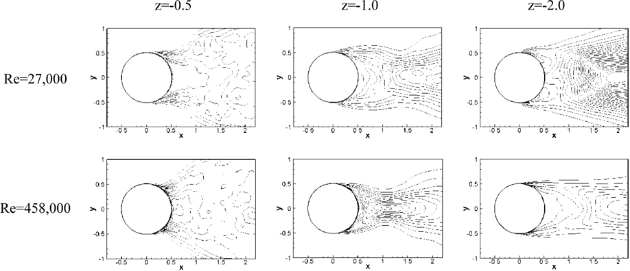
The contours of the mean transverse vorticity are presented in Fig. 16. The mean transverse vorticity is significantly large as the interface approaches. High vorticity magnitudes are observed in the place where the separated region is located and it is related to high interface fluctuations inside separation region. At z = -1 two positive vortices are detached from the cylinder wall and negative vortices are observed near the cylinder for Re = 27,000 while a pair of the symmetric positive vortices forms from the cylinder surrounding the negative vortices for critical Re , which is the recirculation region. Since the transverse vorticity is responsible for the interface fluctuations, much smaller values are observed at z = -2.

Fig. 17 shows the mean vertical vorticity contours. The vertical vorticity is inclined outward in transverse direction from the interface to z = -1. Similar patterns are observed for critical Re with steeper inclined angle. It is also shown that in deep flow the vertical vorticity is created by Karman vortex shedding and the unstable shear-layers behind the cylinder.

Reynolds stresses

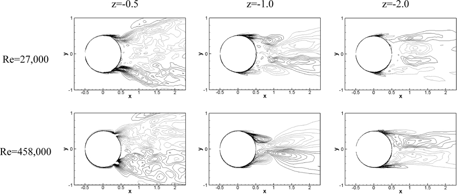
The streamwise Reynolds stress () is shown in Fig. 18. Sub-critical Re (27,000) shows much higher magnitude of than critical and post-critical Re (234,000, 458,000) at all three depths. It is also shown in Singh and Mittal (2005) that sub-critical Re has larger than critical and super-critical Re . The peak values are concentrated on the separated region where very high mean velocity gradients are observed. They are inclined into transverse direction from the interface to about z =-1 as shown Fig. 22 for sub-critical Re and critical Re . The size of wake decreases with Re increase at z = -1 due to the delayed separation point and it gets recovery at z = -2, which is also shown in the mean separation pattern. Fig. 19 presents the mean transverse Reynolds stress (). Near the interface high values of are observed at near separation point and its magnitude shows stronger as Re increases. It is shown that from z = -1 to deep flow achieves a peak along the center axis while the peaks in other Reynolds stresses are located off the flow axis. At z = -1 the peak moves toward into the cylinder as Re increases. However, the peak moves downstream with increase in Re at z = -2. Increased magnitude is observed close to the cylinder especially in the region of separated shear layer as Re increases, indicating an increased unsteady activity in that region of the flow, particularly for critical Re .

The vertical Reynolds stress ( ) is shown in Fig. 20. Three peaks in are observed from the interface to the deep flow as shown in Fig. 22. The maximum magnitudes are observed near the interface for all Re due to the fluctuations of the interface which matches with the first peak from sub-critical Re and critical Re (Fig. 22). The second one is at around z = -1 and this is also seen in Fig. 20 with smaller wake region as Re increases into the critical regime. The features of near the interface are similar with that of .

The mean Reynolds shear stress ( ) is shown in Fig. 21. It is shown that the interface reduces the shear stress remarkably in the wake region (Yu et al., 2008; Suh et al., 2011). For critical Re , much smaller wake region is observed at z = -1 and it recovers at z = -2.

Vorticity transport

Suh et al. (2011) studied the mechanism of the vorticity generation at sub-critical Re (27,000) using the Reynolds-averaged vorticity transport equations which can be obtained by taking curl of the time-averaged Navier-Stokes equation:

where Ω_x , Ω_y , and Ω_z are the streamwise, transverse, and vertical components of the mean vorticity, respectively. Term (A) represents the material derivative of the mean streamwise vorticity. The first term of term (B) is the vorticity amplification by the streamwise stretching and the rest provide vortex-line bending effects. Term (C) represents the vorticity damping by the viscous diffusion, and (D), (E), and (F) are the vorticity production by inhomogeneity in the Reynolds stresses. It is noted that the effect of the air-water interface including the density discontinuity across the interface was neglected.

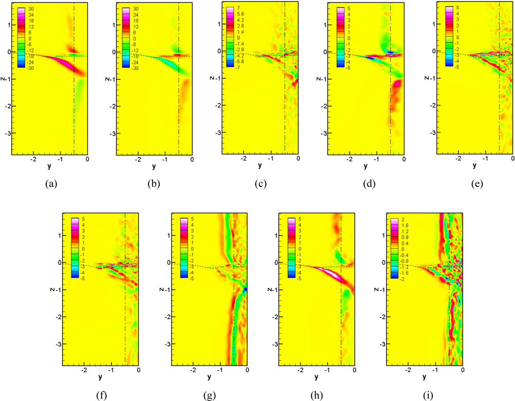
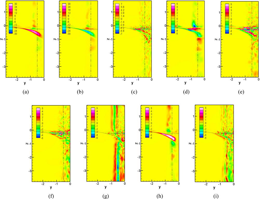
Dominant source terms for the mean vorticity for Re = 27,000 and Re = 458,000 are shown in Figs. 23 and 24 respectively. In the streamwise vorticity equation, the dominant terms are y and z components of term B and term E. The y and z components of term B create the vortex bending whose have a similar magnitude but with opposite signs so they have little effect. The remaining E term, anisotropy term between transverse and vertical Reynolds stress, is mainly responsible for the generation of the mean streamwise vorticity near the interface. This behavior is observed in all Re from sub-critical to critical Re regime.

In the transverse vorticity equation, the dominant terms are z component of term B, E term, and F term. Due to the vortex shedding and shear layer instability, the bending of the vertical vorticity is generated which is the z component of term B. In deep water, the term F is a dominant for the vertical vorticity equations. The z component of the term B is the vortex stretching of the vertical vorticity. The anisotropy term between the streamwise and transverse Reynolds stresses is responsible for the term E.

Overall, for higher Re (234,000, 458,000) the separation point is much delayed compared with that of the sub-critical Re (27,000). Due to the delayed separation, much smaller wake region and smaller separation region are shown for post critical Re .

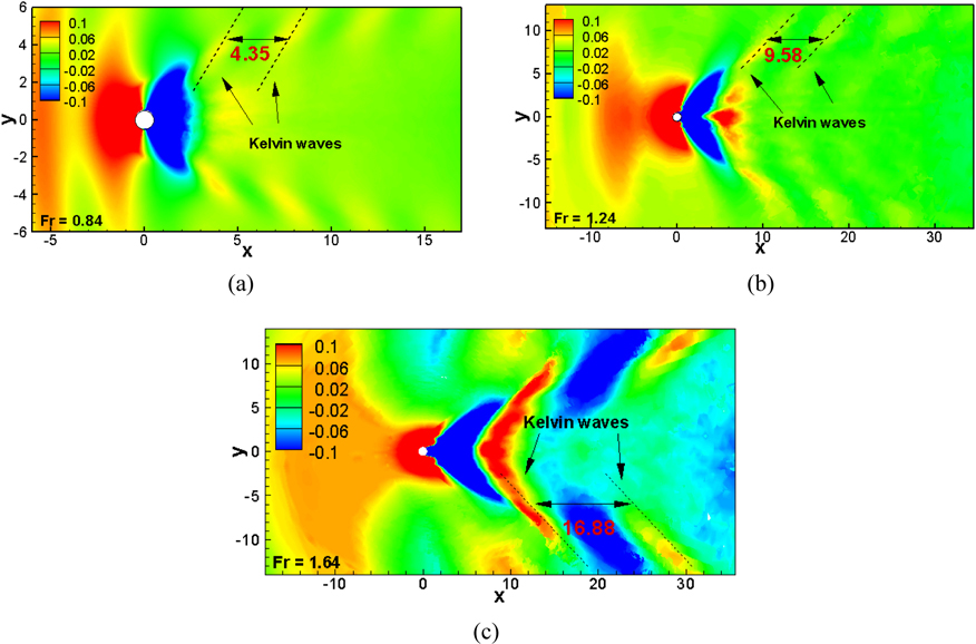
There is little influence of Reynolds number at the air-water interface based on variables related to the air-water interface such as mean interface elevation, run-up height, and Kelvin wave patterns, etc. The instantaneous air-water interface elevations for all different Fr with different Re are shown in Fig. 25. For the lowest Fr (= 0.2), it is hard to see the bow wave in front of the cylinder and small interface deformation is observed in the wake region. For subcritical Fr (= 0.44, 0.84), relatively smaller bow waves are observed in front of the cylinder with Kelvin waves behind the cylinder. There are some free-surface roughness and turbulence in the wake region behind the cylinder. For Fr = 1.24, much increased bow wave is observed and it breaks and wraps around the bow. A lot of splashes and bubbles are intense immediately behind the cylinder. The Kelvin waves are less visible just behind the cylinder due to stronger free-surface oscillations and turbulence. For Fr = 1.64, the bow wave increases remarkably with the largest wake region among four Fr and it also breaks with similar patterns of plunging breakers. Much smaller air-water interface structures including splashes and bubbles are observed behind the cylinder. It is also hard to distinguish the Kelvin waves behind the cylinder due to much larger free-surface oscillations and turbulence.

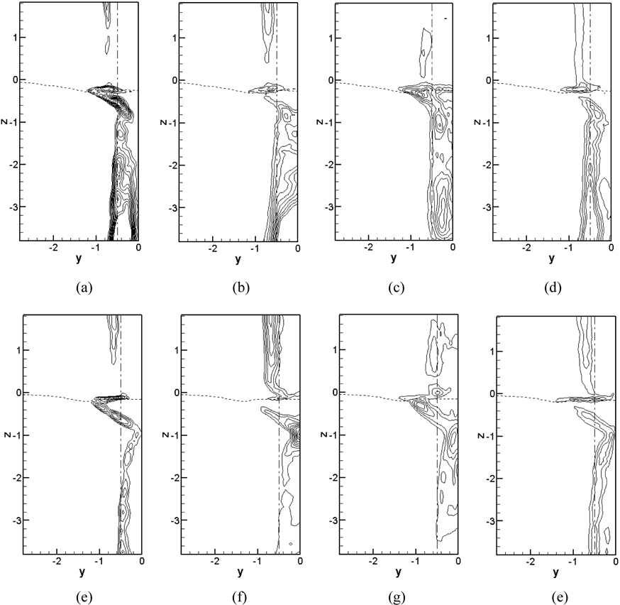
The mean air-water interface elevations (top) are presented in Fig. 26. The time-averaged free surface shows the bow wave in front of the cylinder, depression region or cavity region behind the cylinder, and the diverging Kevin wave. It is also confirmed that the height of the bow wave and the depression depth increases as Fr increases. Except for Fr = 0.2, the diverging Kelvin wave is evident but it is not shown for high Fr (1.24, 1.64) since it is in the far downstream. More details of the diverging Kelvin wave will be discussed later. Fig. 26 also shows the rms of the interface fluctuations (bottom) for different Fr and Re . For low Fr (02.-0.84) as shown in Figs. 26(a), (b) and (c) the fluctuation of the interface starts near the end of the slope from the crest to the surface cavity due to the relatively smaller run-up height and there is almost no fluctuations in front of the cylinder. However, the higher run-up height in front of the cylinder for high Fr cases (Fig. 26(d), (e)) causes the fluctuation from the cylinder front to the depression region. For low Fr (0.2-0.84), the peak value is observed near the edge of the bottom of the depression region, whereas it is shown in further downstream and detached from the cylinder wall for high Fr (1.24, 1.64). In addition, small structures of the interface fluctuation are observed for high Fr due to high Re .

Three different Froude numbers (0.84, 1.24, and 1.64) with Re = 458,000 are investigated to have better understanding of the effect of the air-water interface on the flow structures in the near wake at different Froude numbers. Different Reynolds numbers with above Fr are also compared to examine the Reynolds number dependency. The fine grid solutions will be used for Fr = 1.64 with Re = 458,000 in this study unless otherwise mentioned.

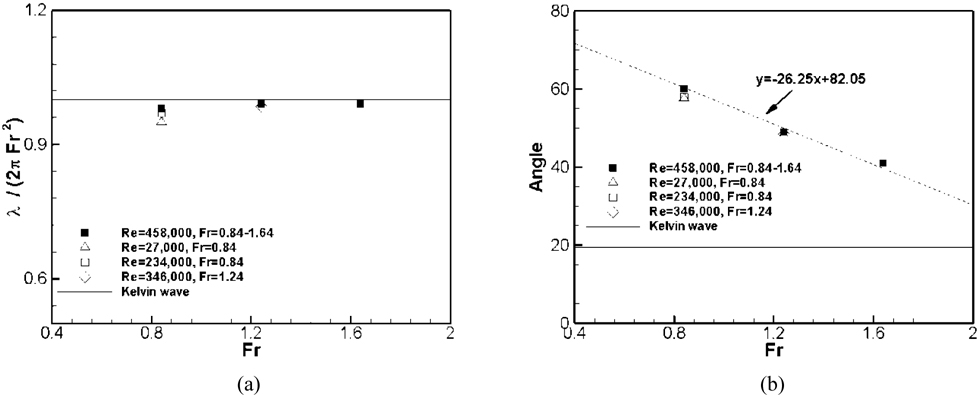
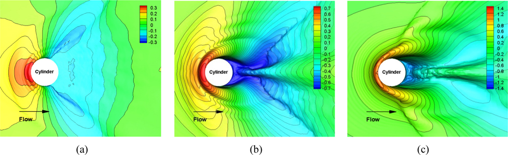
The mean air-water interface elevation contours for all three Fr in Fig. 27 show diverging and transverse wave patterns. The diverging waves are more dominant than the transverse waves with wave lengths that roughly correspond to the theoretical transverse wave length in a Kelvin wave pattern, i.e., λ_t = 2πFr² . The diverging wave lengths for all three Fr match well with theoretical values as shown in Fig. 28(a). In addition, different Reynolds numbers other than Re = 458,000 at Fr = 0.84 and Fr = 1.24 are compared and they show almost similar wave length with ones of Re = 458,000.

The diverging angles for all three Fr are also shown in Fig. 28 and they are all larger than that of the Kelvin wave value (19°) which is typically observed in ship flows. Bhushan et al. (2010) studied the flow around the Air-Cushion Vehicle (ACV) numerically with different Froude numbers and they showed similar Froude number effects that the diverging wave angle of the ACV decreases almost linearly up to Fr = 1.0 and is almost constant thereafter which is within 10% of the Kelvin waves. The flow patterns at high Fr show similar flow features with a slender body whereas the body acts like a blunt object at low Fr . The diverging angles decreases linearly with Fr as shown in Fig. 28(b), which implies that the body looks slenderer as Fr increases due to a cavity region immediately behind the cylinder. In Fig. 28(b), different Reynolds numbers than Re = 458,000 are also added to investigate Re dependency on the free-surface flow and the Re effect is negligible on the diverging wave angle.

Fig. 29 presents the close-up view of the mean air-water interface elevation contours with iso-surface near the cylinder. Contour levels for high Fr (1.64) is 2 and about 5 times greater than those for medium (1.24) and low Fr (0.84), respectively. For Fr = 0.84, the Kelvin waves propagate with a wide angle and relatively small depression depth behind the cylinder. For Fr = 1.24, the depression region immediately behind the cylinder is narrow and deep, which makes the cylinder act like a slender body and this causes smaller diverging angle than that of low Fr . For Fr = 1.64, much larger depression depth is observed and it is even narrower and longer than that of both low and medium Fr , implying that the flow past the cylinder at Fr =1.64 shows features with a slenderer body.

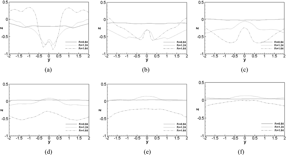
Fig. 30 shows the mean wave profiles at different streamwise locations for three Fr . There is a small and wide depression region behind the cylinder and its recovery is fast for Fr = 0.84. In contrast, it is clearly seen that there is a deep and narrow cavity behind the cylinder for Fr = 1.24 and Fr = 1.64 which is also shown in Fig. 30(b) and (c). The mean wave profile for Fr = 1.24 recovers faster than that for Fr = 1.64, as shown in Fig. 30(d), (e), and (f). A small bump is shown on the centerline y = 0.0 at x = 1.0 for both Fr = 1.24 and Fr = 1.64 and it grows in the streamwise direction up to x = 3.0 and then it starts spreading out to the transverse direction with reduced wave elevation.

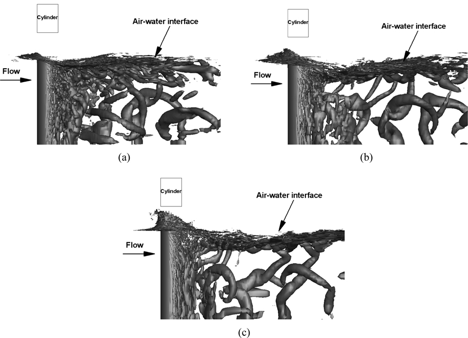
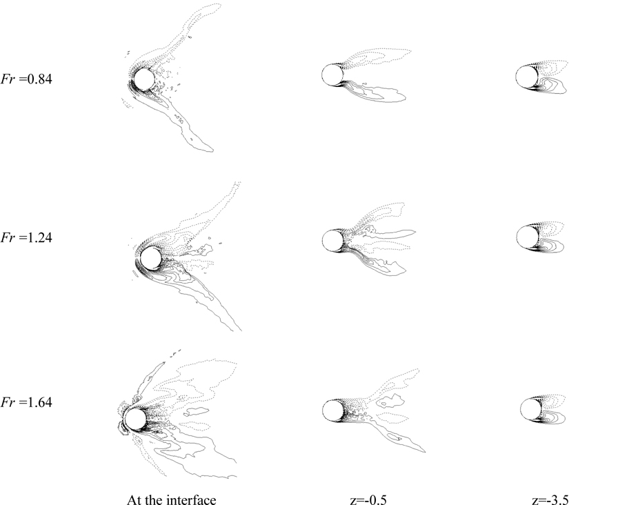
Three-dimensional instantaneous coherent vortical structures identified by the second invariant of the velocity gradient tensor (Hunt et al., 1998) for the three Fr are shown in Fig. 31. At Fr = 0.84, the organized shed vortex tubes are present in the deep flow and they attenuate as the air-water interface approaches. This is consistent with previous work (Suh et al., 2011; Yu et al., 2008). Due to the interface deformations, vortical structures of smaller scales are observed at the air-water interface for all three Fr . At medium and high Fr (1.24, 1.64) small vortical structures near the air-water interface disappear due to the cavity region behind the cylinder and there are only large structures in the deep flow.

Fig. 32 presents contours of the mean vertical vorticity magnitude at different depths for all three Fr . At the air-water interface, the shear layers stretch out with a smaller angle and smaller vertical vortices are observed behind the cylinder as Fr increases. At z = -0.5, the shear layers separate from the cylinder wall and diverge immediately in the transverse direction for Fr = 0.84; whereas for medium and high Fr (1.24, 1.64), the shear layers extend toward the downstream in parallel first and then diverge in the transverse direction. It is clearly shown that a cavity (empty space due to depression depth) behind the cylinder for high Fr makes the cylinder together with its shear layers act like a slender body such that the “separation” of the shear layer occurs away from the real cylinder wall. There is no significant difference in the shear layer pattern and regular vortex streets are observed in the deep flow ( z = -3.5) for all the Fr cases.

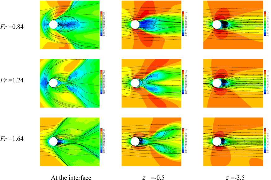
Contours of the mean streamwise velocity with the streamlines are shown in Fig. 33. No remarkable difference in the streamline pattern is observed in the deep flow for all the Fr cases. For low Fr , the recirculation length at the air-water interface is approximately two times of the cylinder diameter while it has much reduced length for high Fr and it has similar size of the cavity behind the cylinder. For both medium and high Fr , counter-rotating vortices are shown immediately behind the cylinder at the interface which is also observed in the deep flow. The streamline patterns for high Fr also confirm that the depression region behind the cylinder acts as a cavity resulting in flow around a slender body.

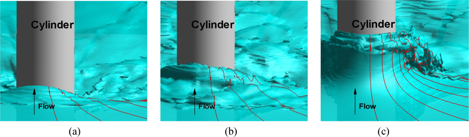
Fig. 34 shows the iso-surface of the air-water interface with slices of the wave profile orthogonal to the cylinder wall for the three Fr . For Fr = 0.84, small disturbances are shown on the interface; however, no breaking waves are observed. For medium and high Fr (1.24, 1.64), the flow becomes unsteady such that small interface structures including splashes and air bubbles are present especially for Fr =1.64 which is also shown in Chaplin and Teigen (2003). The waves arise and break down to the cylinder shoulder as shown Fig. 34(b) and (c), which corresponds to a spilling breaker and a plunging breaker, respectively according to the analysis of Galvin (1968). Similar wave breaking patterns are observed in experimental study of the divergent ship bow waves using eight different Froude numbers by Shakeri et al. (2009) and they showed that for Fr < 1.0 non-breaking waves were generated; spilling breaking waves occurred at between Fr = 1.0 and Fr = 1.3; and plunging breakers were generated at 1.4 < Fr < 1.8.

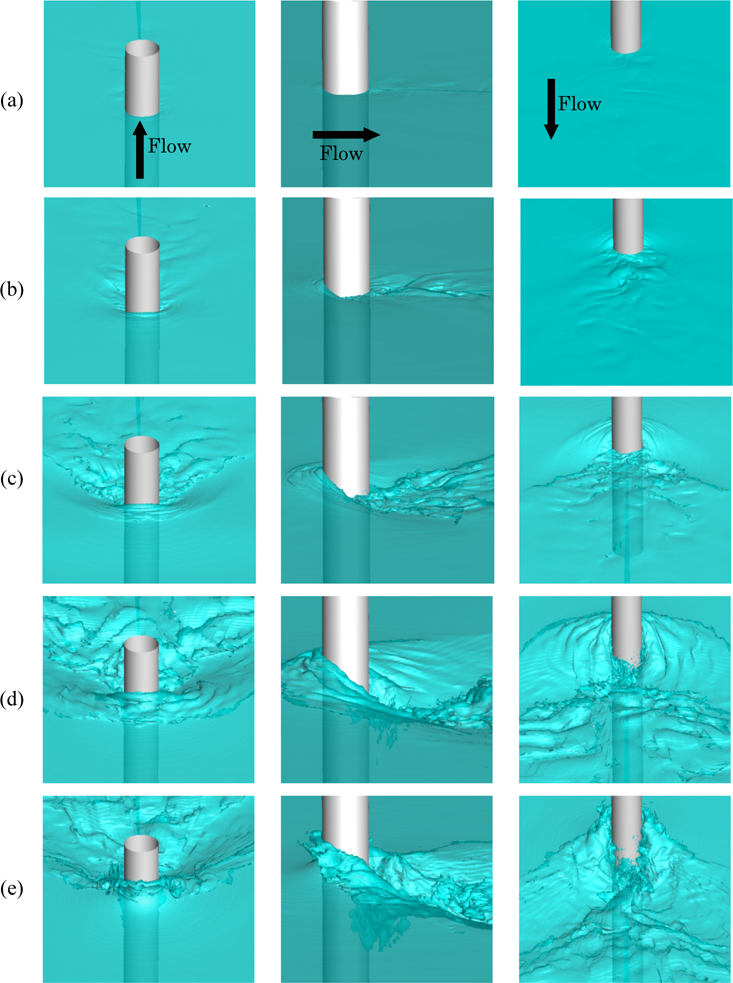
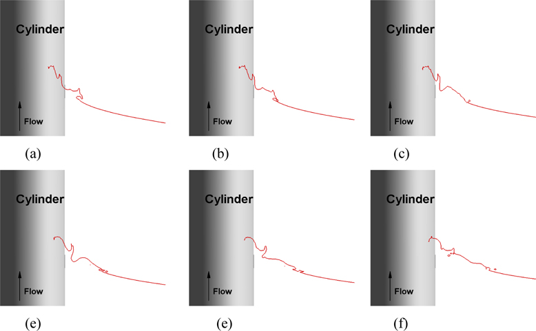
The slices of the wave profile cut for Fr = 1.24 at different circumferential planes, which are presented by the tangential angle θ starting from the downstream direction, are given in Fig. 35 and it demonstrates the spilling wave breaking. In this figure, the flow direction is into the paper which is perpendicular to the cylinder. A small jet grows and starts overturning as shown in Fig. 35(a). It falls into the undisturbed water surface and then a small air entrainment is shown in Fig. 35(b) and (c), respectively. The repeated spilling breaking events including overturning and entrapping air are presented in Figs. 35(d)-(f).

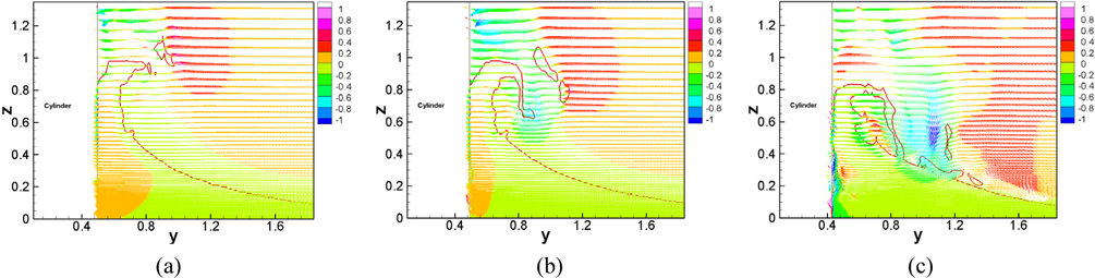
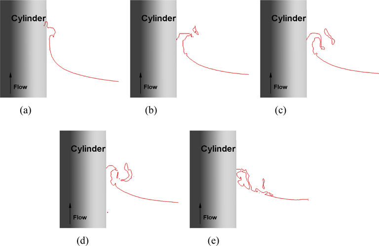
The plunging wave breaking is described in Fig. 36 using the slices of the wave profile cut for Fr =1.64. The wave propagates from the center of cylinder to the cylinder shoulder as shown in Fig. 34(c). When the wave crest grows and starts overturning (Fig. 36(a) and (b)), a jet is stretched and breaks up into droplets before it plunges on the undisturbed water surface (Fig. 36(c) and (d)). After the jet touches the water surface, an oblique splash is created (Fig. 36(e)). These plunging wave breaking events are very similar to those observed in the previous plunging wave breaking literatures (Bonmarin, 1989; Peregrine, 1983; Tallent et al., 1990). However, the direction of the plunging wave breaking is different from the mean flow, which is similar to the numerical simulation of the plunging wave breaking over a submerged bump (Koo et al., 2012) and the numerical study of wave breaking around a wedge-shaped bow (Wang et al., 2010). It should be mentioned that the wave plunges forward in the same direction of the mean flow for most previous studies on plunging wave breaking. The shape of the plunging jet is an ellipse with aspect ratio 1.8 which is close to the findings from most previous studies ( ). The thickness of the jet is approximately 0.012 and the similar jet thickness is reported in the experimental studies (Bonmarin, 1989; Grue and Jensen, 2006; Kimmoun and Branger, 2007). The jet angle relative to the undisturbed water surface is about 67° which is larger than that from previous experimental and computational studies on the plunging wave breaking.

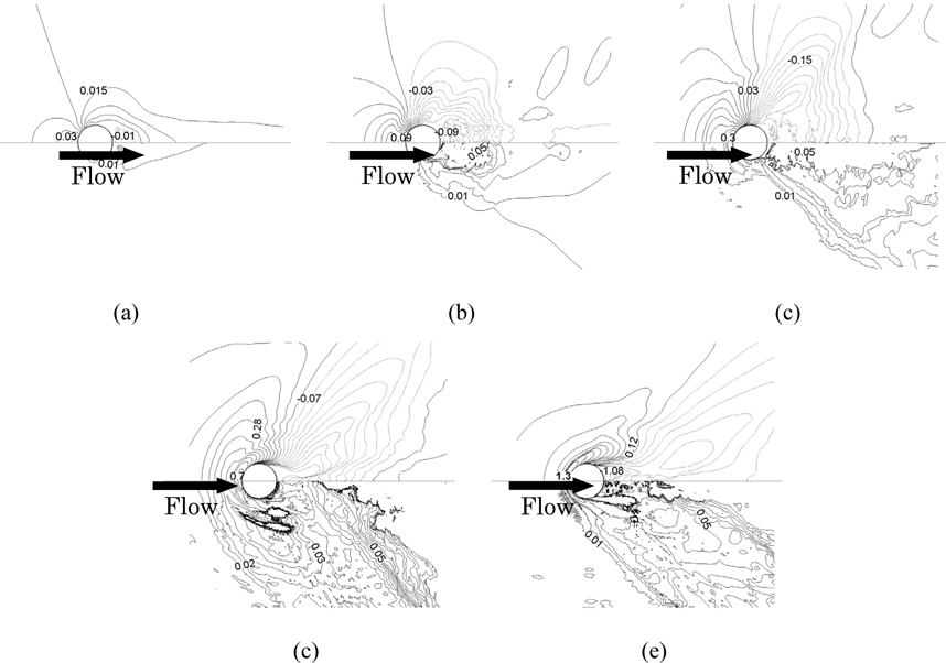
The velocity vectors of the plunging jet are given in Fig. 37 with the colored vectors by the vertical velocity component. Strong air flows are induced by the overturning motion of the jet as shown in Fig. 37(a) and (b), resulting in a pair of vortices immediately before the overturning jet. After the jet touches the interface, a strong vortex is created as a result of the entrained air and small vortices are also produced due to splashes as shown in Fig. 37(c).

In summary, for the Fr effect in fixed post-critical Re = 458,000, it is shown that the length of Kelvin wave increases with Fr ; much less vertical structures are obtained near the air-water interface for post-critical Fr ; much larger cavity is formed behind the cylinder for Fr =1.24 and 1.64 and the flow behind cylinder becomes very different from that of Fr = 0.84; and wave breaking is observed for higher Fr (1.24 and 1.64) while there is no wave breaking for Fr = 0.84.

The two-phase turbulent flow past an interface-piercing circular cylinder at different Reynolds and Froude numbers is studied numerically using large-eddy simulation with a Lagrangian dynamic subgrid-scale model. Verification and validation studies are performed to show the accuracy of the simulations with comparisons against available experimental data.

It is found that the variation in sub-critical Re has small influence for fixed sub-critical Fr . Current results for sub-critical Re with fixed sub-critical Fr show similar trends with Suh et al. (2011) on run-up height, depression depth, mean surface elevation, and mean streamwise velocity.

The flow features near the air-water interface show significant changes with different Reynolds numbers from sub-critical to post critical regime at Fr = 0.84. The present simulations show that the interface makes the separation point more delayed for all regimes of Re . Remarkably reduced separated region below the interface at z = −1 was observed for the critical Re regime and it is responsible for much reduced wake and recirculation region behind the cylinder and it recovers in the deep flow.

The present study shows that the air-water interface structures are remarkably changed with different Froude numbers. For sub-critical Fr, relatively smaller bow waves are observed in front of the cylinder with Kelvin waves behind the cylinder and small amount of free-surface roughness and turbulence are also seen in the wake region. For Fr =1.24 , much increased bow wave is observed and it breaks and wraps around the bow. A lot of splashes and bubbles appear immediately behind the cylinder. Stronger free-surface oscillations and turbulence makes Kelvin waves less visible. For Fr =1.64 , the bow wave increases remarkably with the largest wake region and deepest depression and it also breaks with similar features of plunging breakers which are also shown in previous studies of plunging wave breaking. Much smaller air-water interface structures including splashes and bubbles were observed behind the cylinder. It is also hard to distinguish the Kelvin waves behind the cylinder due to much larger free-surface oscillations and turbulence. As Fr increases, the Kelvin wave angle decreases and deeper and narrower depression region behind the cylinder were observed. This cavity region behind the cylinder makes the cylinder resemble a slender body so that the flow features are significantly different that around the cylinder.

Recently, the 27th International Towing Tank Conference (ITTC) Ocean Engineering Committee (2013) conducted a workshop on wave run-up and vortex shedding on cylinders. Participants submitted results for specified conditions without access to the experimental validation data prior to the workshop. Subsequently the participants were provided the experimental data and will submit final results. The authors submitted results for both test cases (Yoon et al., 2013; Yeon et al., 2013). Relevant to the present research are the results submitted for the vortex-shedding test case, which covered sub, critical and post critical Re for single-phase conditions using the same computational method as used herein, but without air-water interface and investigations of effects of aspect ratio/span length, conservative vs. non-conservative convection schemes, and grid resolution. Highest accuracy predictions for sub, critical and post critical Re required aspect ratio of 8 for sub critical vs. 2 for critical and post critical Re ; conservative convection schemes for critical and post critical Re ; and much finer grids with 67 million grid points. The present simulations for the deep flow have limitations in this regard along with free surface effects for larger Fr. The available experimental data for critical and post critical Re and Fr is also limited, as previously discussed. Thus, additional two-phase surface-piercing cylinder experimental and numerical studies for critical and post critical Re and Fr are required to confirm the effects of both Re and Fr . However, unless very large experimental facilities are used it will be difficult to achieve sufficiently large aspect that the deep flow is unaffected by the free surface and has sufficient additional span length for canonical single-phase flow without blockage effects, especially for sub and critical Re.