The application of friction stir welding (FSW) technology has been extended to all industries, including shipbuilding. A heat transfer analysis evaluates the weldability of a welded work piece, and elasto-plastic analysis predicts the residual stress and deformation after welding. A thermal elasto-plastic analysis based on the heat transfer analysis results is most frequently used today. However, its application to large objects such as offshore structures and hulls is impractical owing to its long computational time. This paper proposes a new method, namely an equivalent strain method using the inherent strain, to overcome the disadvantages of the extended analysis time. In the present study, a residual stress analysis of FSW was performed using this equivalent strain method. Additionally, in order to reflect the external constraints in FSW, the reaction force was predicted using a neural network, Finally, the approach was verified by comparing the experimental results and thermal elasto-plastic analysis results for the calculated residual stress distribution.
Friction stir welding (FSW) was invented in 1991 at The Welding Institute, and nowadays is widely utilized in the shipbuilding, aerospace, rolling stock, automobile, construction, electrical, machinery and equipment industries(Thomas et al., 1991; Thomas et al., 1993; ESAB, 2011). FSW has many advantages, a discussion of which is available in the literature(Kang and Jang, 2014). With the extension of the application of the FSW technique across multiple industries, several problems have begun to arise. One of them is related to residual stress. FSW being solid-state welding, the heat input is small; thus, compared with conventional welding, residual stress and welding deformation are also small. Since angular distortion is negligible, the temperature gradient of the upper and lower surfaces, correspondingly, is small as well. Only transverse shrinkage occurs, but this is also small. However, unlike the case of welding deformation, residual stress is not negligible, because the weld zone temperature is about 80-90% of the FSW melting point. In the relevant previous studies, residual stresses were measured at about 60-98.5% of the yield stress(Feng et al., 2004; Han et al., 2011; Steuwer et al., 2006; Lemmen et al., 2010). Additionally, the problems related to residual stress were reported in other studies.(Chen and Kovacevic, 2006; Chuan and Xiang, 2013; Kumar et al., 2013). For prediction and control of welding deformation and residual stress, the thermal elasto-plastic analysis method is widely employed. The best advantage of this method is the accuracy of its result. However, it requires huge computational time as the number of elements increases, owing to its non-linear analysis.
In order to overcome the problem of huge computational time, several simplified assessment techniques such as the equivalent load method and the equivalent strain method, based on inherent strain, have been proposed since the 1980s. The equivalent load method(Kim et al., 2012; Lee, 2010; Ha et al., 2007; Kim and Jang, 2003) and the equivalent strain method(Kim, 2010; Kim, 2014) have been mainly applied to steel. Using the equivalent load method, Jang and Jang(2010) and Mun and Seo(2013) carried out FSW deformation analyses. However, as noted above, the welding deformation is negligible, whereas the residual stress is significant. In the present study, FSW residual stress is calculated using the equivalent strain method and compared with thermal elasto-plastic analysis and experimental results. In FSW, a reaction force is generated by external constraint, which is one of the important input to inherent strain method. The reaction force can be calculated through elasto-plastic analysis, but normally it costs too much computation time and dose not satisfy the original purpose of inherent strain method. Therefore, this study proposes another simple method to predict the reaction force. In the present study, reaction force is predicted using neural networks(Priddy and Keller, 2005). Neural networks solve problems in a manner similar to the human brain: To process a signal, neurons are connected to the neuronal tissue that is part of the basic structure of the brain; likewise, a neural network is a mathematical model of neuronal connections. In order to distinguish this mathematical neural network from the natural biological one in the brain, it is referred to as an artificial neural network. This, as an interconnected network of simple processing elements, is a powerful data modeling tool for capturing and representing complex input and output relationships. Finally in the present study, the reaction force is predicted, and its effect in the unit inherent strain analysis model is considered.
This paper unfolds as follows. In section 2, details of the experiment condition are explained. Section 3 provides the equivalent strain method using inherent strain procedure. In section 4, detailed prediction of reaction force using neural networks is provided. Section 5 provides a comparative study results to verify the proposed method. Conclusion is laid in section 6.
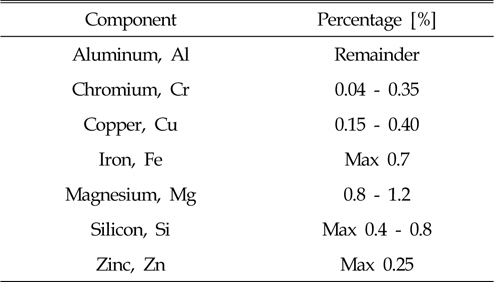
In this study, butt FSW experiments are carried out using aluminum alloy 6061-T6. The chemical constituents of this alloy are listed in Table 1.
[Table 1] Chemical composition of aluminum alloy 6061-T6

Chemical composition of aluminum alloy 6061-T6
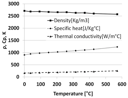
To calculate the temperature field, material nonlinear and thermal conductivity. These material properties are plotted in Fig. 1(Chao and Qi, 1998).
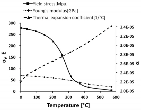
The temperature dependent yield stress, Young's modulus and coefficient of thermal expansion are applied to the structural analysis as shown in Fig. 2(Chao and Qi, 1998).
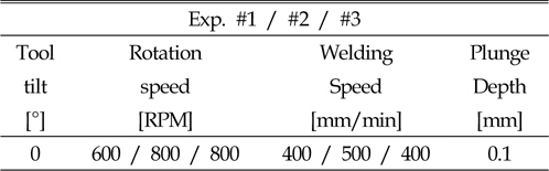
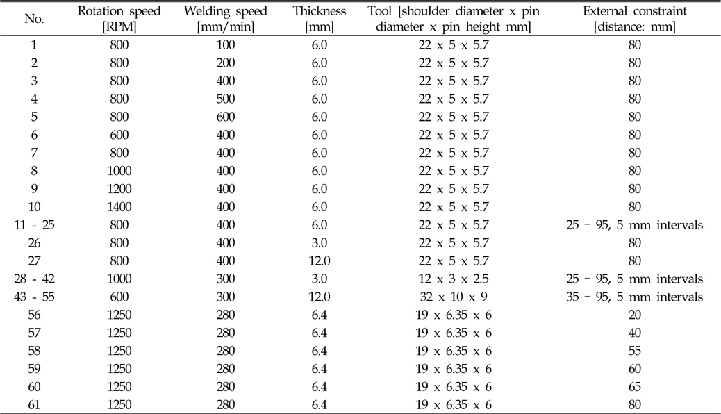
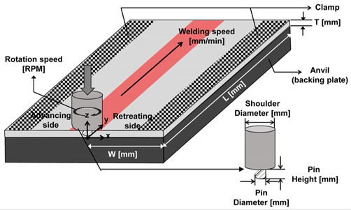
The work piece and the tool dimensions are listed in Table 2, and the welding parameters are provided in Table 3. The specified thickness 6mm in Table 3 for aluminum alloy 6061-T6 has a good weldability during FSW.
[Table 2] Work piece and tool dimensions for experiments
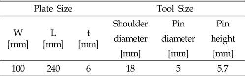
Work piece and tool dimensions for experiments
[Table 3] Welding parameters of experiments

Welding parameters of experiments
A detailed experimental schematic diagram is shown in Fig. 3.
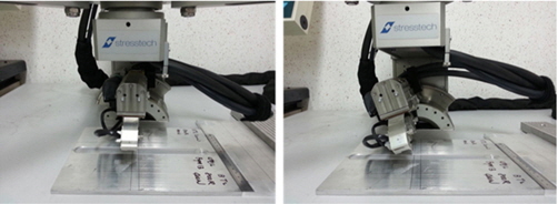
After finishing the FSW, the residual stress is measured by X-ray diffraction methods. The X-ray diffraction equipment is the XSTRESS3000 model(Stresstech Group, 2007) as shown in Fig. 4.
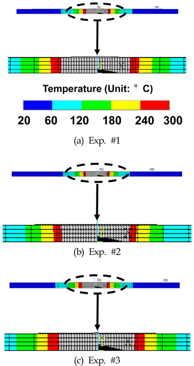
In order to investigate the asymmetric effect of FSW, the residual stress is measured at the advancing and retreating sides. The measured line is perpendicular to the weld centerline, which is located 100 mm far from the starting point of welding in the y-direction. The measured points of residual stresses are located at 0 - 20 mm with 1 mm intervals, 20 - 50 mm with 5 mm intervals, and 50 - 100 mm with 10 mm intervals relative to the weld centerline. Also, the residual stress is measured in the longitudinal and lateral directions of the weld.
3. Equivalent strain method using inherent strain
3.1 Definition of inherent strain
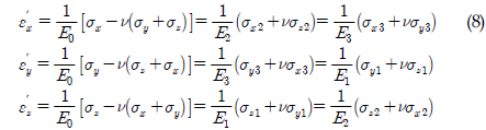
During the welding process, the total strain is divided into four kinds of strains: elastic strain, plastic strain, thermal strain, and phase transformation strain. The inherent strain is the difference between the total strain and the elastic strain. Thus, it can be expressed as the following Eqs. (1)-(2).


where
3.2 Three dimension solid-spring model
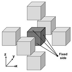
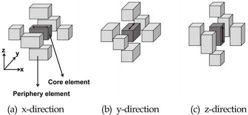
A weld joint region expands or shrinks due to welding process. At this time, periphery is also effected by weld joint region. Mainly restraining elements against the expansion of core element in each of three directions are depicted in Fig. 5.
Three dimension solid-spring model is assumed to be axis symmetric. Because coefficients of thermal expansion has the same values in all directions. To prevent a rigid body motion without disturbing the intended structural behavior, one side of each axis is fixed, and the other side is allowed to move along the axis as shown in Fig. 6.
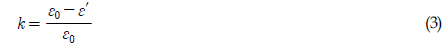
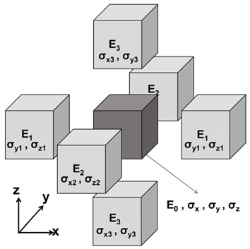
The elastic modulus of the periphery element to induce the temperature changes and restraint is determined through the following process(Kim, 2014). The elastic modulus and stresses of core and periphery elements are defined as depicted in Fig. 7. Where core element is subjected to restraint by the periphery elements. The degree of restraint is Eq. (3):

where
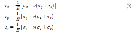
The unit stress 𝜎0 is applied to the model, the unknown stresses are defined such as 𝜎

where 𝜎

Eq. (5) can be expressed as Eq. (6) in a free body state. Each of the axial stresses has the same value.

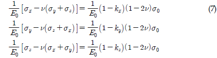
Eq.(7) can be expressed by using Eqs.(3), (5), and (6).

Since the strain of the core element is the same as those of periphery elements, as explained by the definition of the restraint model, the following equations are derived.
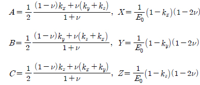
The elastic modulus of the periphery element is calculated follows by Eqs.(7)-(8).

where
3.3 Factors affecting inherent strain
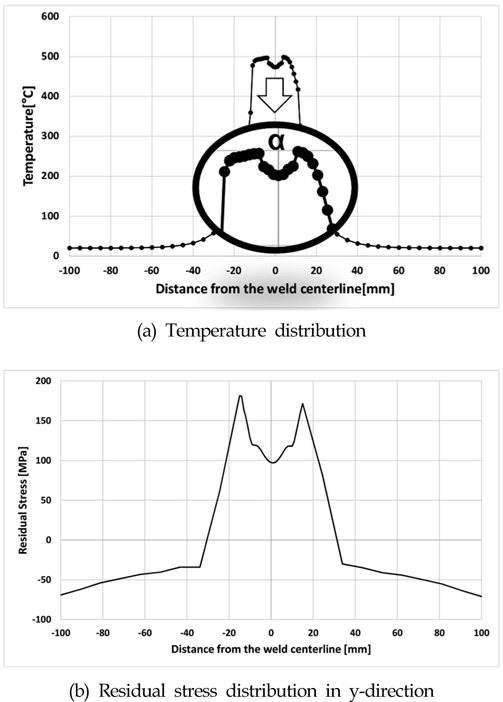
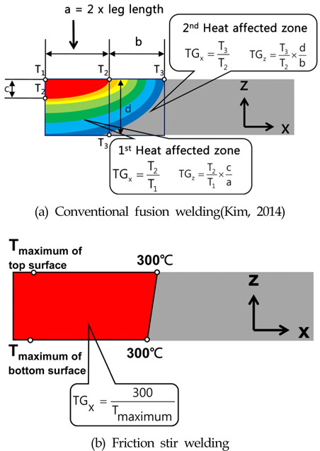
Inherent strain is affected by several factors including maximum temperature, temperature gradient in three directions, restraint, external constraint, etc. Kim(2010) considered maximum temperature and restraint in calculating inherent strain, whereas Kim(2014) suggested that maximum temperature, temperature gradient in three directions, and external constraint are the most important factors in calculating inherent strain. Restraint has a small effect on inherent strain, whereas temperature gradient in three directions and external constraint have large effects(Kim, 2014).
A heat transfer analysis is carried out using Fluent(Fluent Inc., 2006), a commercial computational fluid dynamics program. After the heat transfer analysis, the maximum temperature and temperature gradient are calculated. The temperature gradient is represented by an index named
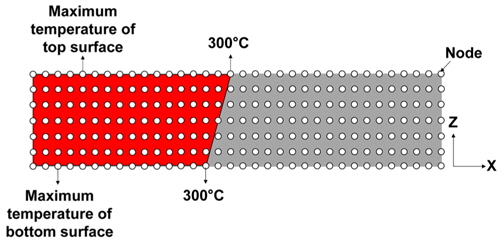
There is almost no temperature gradient between the top and bottom surfaces (during FSW, heat is applied not only to the top surface but to the bottom surface). Thus, there is almost no angular distortion due to the temperature gradient of the top and bottom surfaces. The work piece expands laterally during heating, and then contracts during cooling. Thus,
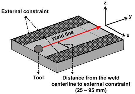
In the previous study by Kim(2014), the value of the external constraint was not defined. In the present study, the value of the external constraint is defined as the distance from the weld centerline, as shown in Fig. 9.
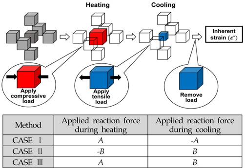
Generally, the external constraint is applied until the work piece temperature reaches room temperature. It prevents movement of the work piece and welding deformation. At this time, reaction force arises in the external constraint. Thus, inherent strain is calculated for the existing external constraint in the heating and cooling stages. In the vicinity of the joint region, an x-direction compressive and tensile loads are added during the heating and cooling stage of FSW, respectively. After the temperature of the work piece reaches room temperature, the x-direction load is removed. Residual strain at this stage is the final inherent strain.
The reaction force is different during heating and cooling. Generally, it greatly affects inherent strain during the cooling stage. However, there is a serious problem in calculating reaction force, because it is calculated by thermal elasto-plastic analysis. Thus, an alternative method for prediction of reaction force is required. Before predicting the reaction force however, its effect on the residual stress distribution during heating and cooling is determined by thermal elasto-plastic analysis.
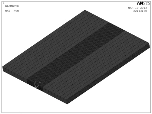
61 times different thermal elasto-plastic analyses are carried out in total using ANSYS (ANSYS Inc., 2011). The work piece and the tool dimensions are listed in Table 2 and finite element(FE) model is shown in Fig. 10.
Steady state heat transfer analysis is carried out in Eulerian description, and then the results are transferred to the FE model, for elasto-plastic analysis. Transient heat transfer analysis is performed in the FE model, and the temperature is assumed as quasi-steady state during the welding process. At this time, the temperature data is extracted in heat source region with 1 mm interval, and transferred to the FE model nodes. The definition of heat source region in CFD model is referred to previous literature(Kang et al., 2014)
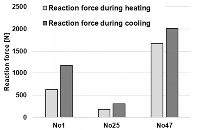
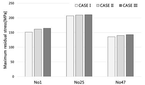
The relevant welding conditions and parameters are listed in Table. 4. The most serious three cases (No. 1, No. 25, and No. 47) were chose to compare differences of the residual stress distribution between thermal elasto-plastic analysis and the inherent strain method. The case of No. 1 shows the largest reaction force difference between heating and cooling. The cases of No. 25 and No. 47 shows small and large reaction forces, respectively.
[Table 4] Welding conditions and parameters for thermal elasto-plastic analysis

Welding conditions and parameters for thermal elasto-plastic analysis
The reaction forces during heating and cooling in the No. 1, No. 25, and No. 47 cases are plotted in Fig. 11.
In this study, three different methods are employed to calculate inherent strain. The reaction force during heating and cooling is assumed as
3.5 Location of inherent strain input
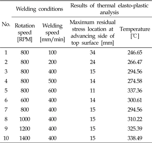
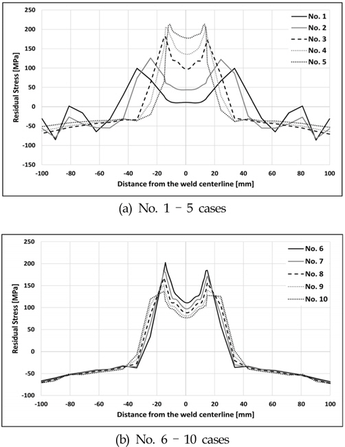
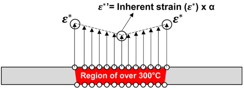
In Table 5, the locations of maximum tension residual stress in the y-direction are presented for No.1 – No.10 cases. As a result, the location of maximum tension residual stresses are found near 300℃, as indicated in Fig. 13 and Table 5.
[Table 5] Maximum residual stress locations at advancing side of top surface for No. 1 - 10

Maximum residual stress locations at advancing side of top surface for No. 1 - 10
Actually, the
In the previous study by Kim(2014), the welding analysis model was divided into two regions, that is, the 1st and 2nd heat-affected zones, depending on the level of the temperature variation. Then, the
Inherent strain is calculated using the maximum temperature,
The ratio between the center and edge of the tool is defined as α, as shown in Fig. 16(a), and is multiplied by the inherent strain. This fixed inherent strain is defined as
3.6 Residual stress distribution according to reaction force in thermal elasto-plastic analysis
The residual stress distribution is calculated by elastic structural analysis with the inherent strains for No. 1, No. 25, and No. 47. The maximum tensile residual stresses in the y-direction are compared in Fig. 18.
In Fig. 18, the inherent strain during cooling is more important than the heating process. The CASE II and CASE III results are almost the same, which means that the inherent strain is produced during cooling. This is why the yield stress during the cooling stage is higher. Finally, we decide to use of the reaction force during the cooling stage as representative one.
4. Prediction of reaction force using neural networks
4.1 Factors affecting reaction force
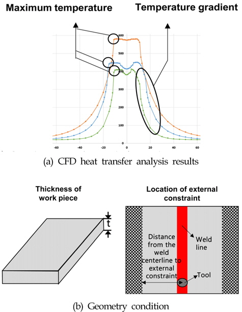
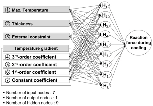
In this study, welding speed, rotation speed of tool, and tool dimensions are represented by the maximum temperature and temperature gradient. Thus, the input data can be summarized as shown in Fig. 19.
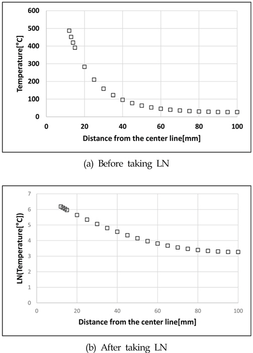
In order to quantify the temperature gradient, it is approximated using a third-order polynomial function. However, in consideration of the maximum temperature, it is difficult to approximate temperature gradient data by a trend line. Maximum temperature is already considered as a factor in calculating the reaction force using neural networks. Thus, maximum temperature is no more necessary in the temperature distribution graph. Taking the natural logarithm on the temperature distribution data, a shown in Fig. 20, the slope of the graph changed less stiff.
4.2 Structure of neural networks
The neural network structure is used to predict the reaction force during the cooling stage, as shown in Fig. 21.
In the figure, the number of nodes in the input layer, in the output layer, and in the hidden layer are 7, 1, and 9, respectively. In general, the number of nodes in the hidden layer is equal to or greater than the sum of the nodes in input and output layers(Priddy and Keller, 2005).
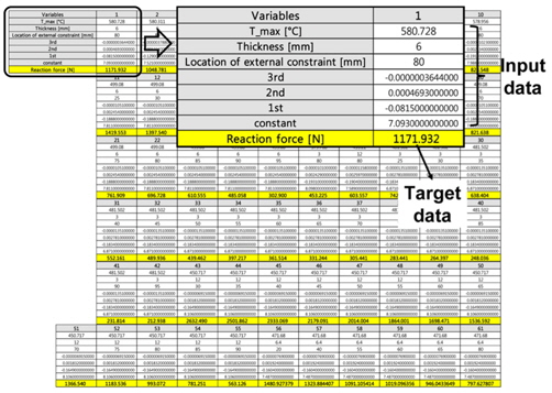
A thermal elasto-plastic analysis are carried out for 61 cases in total in order to make a neural networks function. The relevant welding parameters are summarized in Table 4. Then, the input data and output data are arranged as shown in Fig. 22.
4.3 Verification of neural networks function
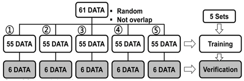
Of the databases constructed, 55 cases are randomly selected for training of the neural network. Then, using the data of the remaining six cases, the function of the neural networks is verified. This procedure is repeated five times, as shown in Fig. 23. Finally, it is confirmed that the input valueis appropriate for prediction of the reaction force during the cooling stage using the neural networks. The verified results are listed in Table 6.
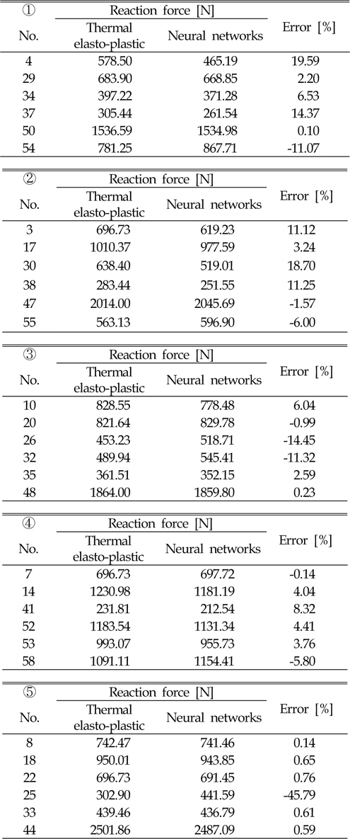
Comparison of thermal elasto-plastic analysis and neural networks results for reaction force during cooling stage
As shown in Table 6, the prediction of the reaction forces during the cooling stage using the neural networks is suitable.
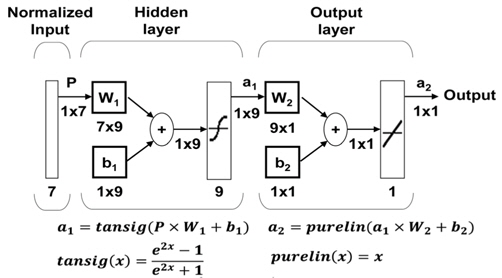
In order to implement the neural networks, 'Neural Network Toolbox in MATLAB' is used(Demuth and Beale, 1998). After completing the verification of effectiveness of the neural networks, the final neural network function is trained using the 61 databases.
Maximum temperature, thickness, external constraint, and temperature gradient (coefficients of third-order polynomial expression) are needed for input data. Reaction force during cooling (output data) is predicted by using the neural networks function shown below. Thus, thermal elasto-plastic analysis can be replaced by neural network prediction of reaction force. The final neural networks structure is shown in Fig. 24.
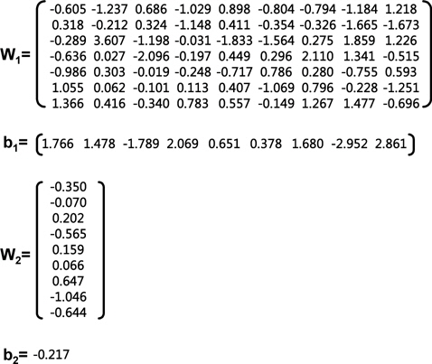
The weight and bias matrices for reaction force during the cooling stage are listed in Table. 7.
[Table 7] Weight and bias matrices for reaction force during cooling

Weight and bias matrices for reaction force during cooling
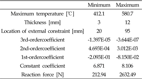
When using this neural networks function, the input and output data have to be normalized. Table 8 lists the normalized minimum and maximum values of input data used. Most of the general FSW experimental conditions are included in the table.

Minimum and maximum values of input data for 61 databases according to thermal elasto-plastic analysis results
However, the new input and output data should be generated for the new FSW experimental conditions, it is alternatively possible to utilize Fig. 24, Table 7 and Table 8 to predict the reaction force during cooling, when we have no data from thermal elasto-plastic analysis.
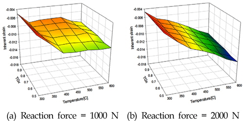
Inherent strain charts considering external constraint are calculated using maximum temperature, temperature gradient, and reaction force. The temperature gradient is divided into
5. Analysis results and discussion
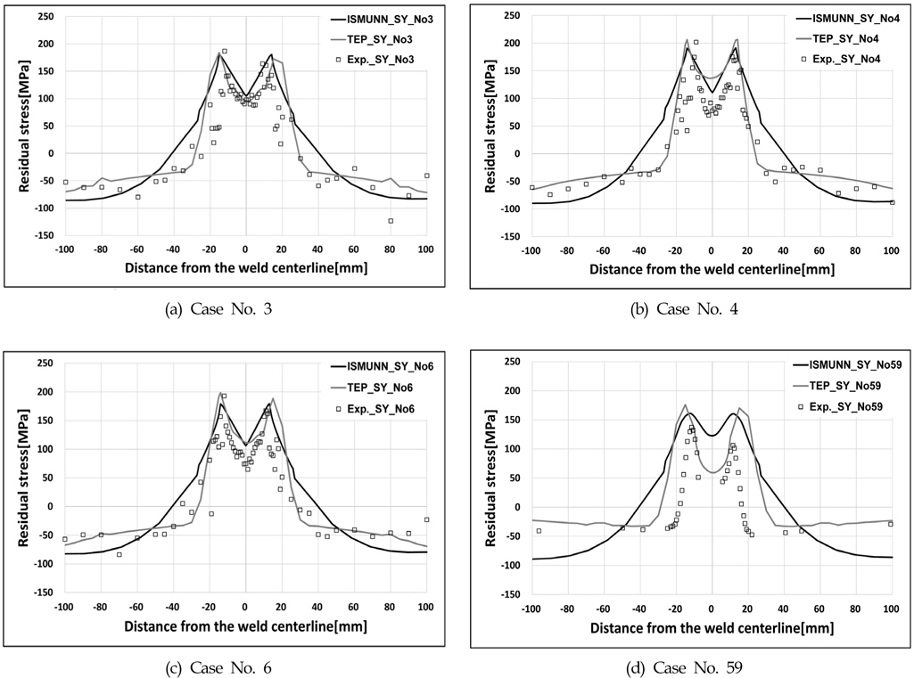
Four cases of the calculated residual stress in y-direction are compared in Fig. 26. with different ways, i.e. experimental data, thermal elasto-plastic analysis, and inherent strain method using the neural networks, respectively.
In Fig. 26 (d), the experimental residual stress data is obtained from a previous study(Feng et al., 2004). According to the results, it is possible to verify the position and value of the residual stress distribution in the y-direction when compared with experimental data, thermal elasto-plastic analysis, and inherent strain method using neural networks are almost identical. Additionally, the alpha was introduced to calculate the residual stress distribution in the y-direction of the featured 'M-shape'. Roughly, the inherent strain method using neural networks and the experimental results are consistent in the vicinity of the weld. However, there is a limitation to the prediction of the residual stress in the peripheral region of the tool by the introduction of alpha. This is why in the weld, empty space occurs in work piece when the tool has passed over to the stirring. Furthermore, downward force is applied to the base material during FSW. Therefore, some error is incurred when comparing the analysis results with the experimental results. Nevertheless, the experimental residual stress distribution y-direction results and other simulation results show good agreement in each case. Therefore, it is verified that the proposed FSW residual stress analysis based on the inherent strain method using neural networks is a reasonable method.
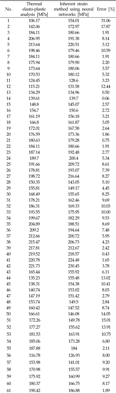
Using this method, the maximum residual stress values in the y-direction in 61 cases in Table 4 are compared in Table 9.
[Table 9] Maximum residual stress in y-direction

Maximum residual stress in y-direction
In Table 9, 52 cases have an error of 10% or less, 8 cases have an error of 10 - 20%, and only 1 case had an error of over 20%. In the case of the over-20% error, the maximum tensile residual stress is located at about 250℃. However, for consistency, it is considered that the inherent strain should be inputted in the 300℃ position. For this reason, a large error occur between the thermal elasto-plastic analysis and the inherent strain method. Overall though, the residual stress results of the elasto-plastic analysis and inherent strain method show fairly good agreement.
In the present study, an FSW analysis based on the equivalent strain method to cover external constraint is carried out according to the computational fluid dynamics analysis result.
The factors affecting inherent strain values are maximum temperature, temperature gradient (
Finally, the experimental and thermal elasto-plastic analysis results are compared with that of the inherent strain method. Significantly, the residual stress distribution show fairly good agreement.