Through-silicon vias (TSVs) are fine, deep holes fabricated for connecting vertically stacked wafers during three-dimensional packaging of semiconductors. Measurement of the TSV geometry is very important because TSVs that are not manufactured as designed can cause many problems, and measuring the critical dimension (CD) of TSVs becomes more and more important, along with depth measurement. Applying white-light scanning interferometry to TSV measurement, especially the bottom CD measurement, is difficult due to the attenuation of light around the edge of the bottom of the hole when using a low numerical aperture. In this paper we propose and demonstrate four bottom CD measurement methods for TSVs: the cross section method, profile analysis method, tomographic image analysis method, and the two-dimensional Gaussian fitting method. To verify and demonstrate these methods, a practical TSV sample with a high aspect ratio of 11.2 is prepared and tested. The results from the proposed measurement methods using white-light scanning interferometry are compared to results from scanning electron microscope (SEM) measurements. The accuracy is highest for the cross section method, with an error of 3.5%, while a relative repeatability of 3.2% is achieved by the two-dimensional Gaussian fitting method.
With increasing use of smart mobile devices such as smartphones and tablets, many electronic components of semiconductors must be smaller and perform multiple functions. Three-dimensional (3D) packaging technology that stacks wafers vertically has been suggested to meet these requirements. To connect the stacked wafers electrically, high-aspectratio holes filled with conductive material in silicon wafers are essential to this 3D packaging process.
Manufacturing faults such as electrical disconnection between stacked wafers and problems in the package bonding process can occur due to the geometrical inaccuracy of TSVs, for example, shorter or longer holes than specified. Asymmetric shapes, different sizes of holes, and improperly filled conductive materials can also cause problems. The measurement of depths and diameters of TSVs is very important for the monitoring process during fabrication. Some researchers have tried to measure the depths and diameters of TSVs using scanning electron microscopes [1], infrared (IR) microscopes [2-4], diffraction phenomena [5], laser interferometry [6, 7], reflectometry [8, 9] and white-light interferometry [10, 11]. There has been, however, very little research on the critical dimension of the bottom part of the TSV, that is, the bottom CD.
In this paper we apply white-light scanning interferometry and propose four bottom CD measurement methods for TSVs. Three of them are direct measurement methods that use original measurement data, such as 3D surface data and tomographic image data, while the fourth is a postprocessing method using a modeling technique to improve the relative repeatability of the CD measurement. Although a direct measurement method is easy to use for calculating the CD, the relative repeatability is quite low, because the original measurement data is deteriorated by the structural characteristics of these TSVs. The high aspect ratio causes reflected light to experience large attenuation around the edge of the bottom of the TSV, in spite of using low numerical aperture interferometry. For this reason the 3D surface data can be distorted from the actual shape, and the edge lines of the bottom tomographic image can be blurred, which worsens the measurement repeatability. To improve the relative repeatability of the measurement, a postprocessing method using a two-dimensional Gaussian fitting model is proposed.
The original measurement data are acquired using low numerical aperture white-light scanning interferometry, and the performance of each proposed measurement method is evaluated in terms of its accuracy and relative repeatability.
II. BOTTOM CD MEASUREMENT METHODS
In this section we propose four kinds of bottom CD measurement methods for TSVs using low numerical aperture white-light scanning interferometry. The cross section method, profile analysis method, and tomographic image analysis method are proposed as direct measurement methods, calculating the diameter of the TSV using original measurement data, such as 3D surface data and tomographic image data, plus least-squares circle fitting, as shown in Appendix A. A two-dimensional Gaussian fitting method using converted 3D surface data for the TSV bottom tomographic image is proposed as a postprocessing method to improve the relative repeatability of the direct measurement methods.
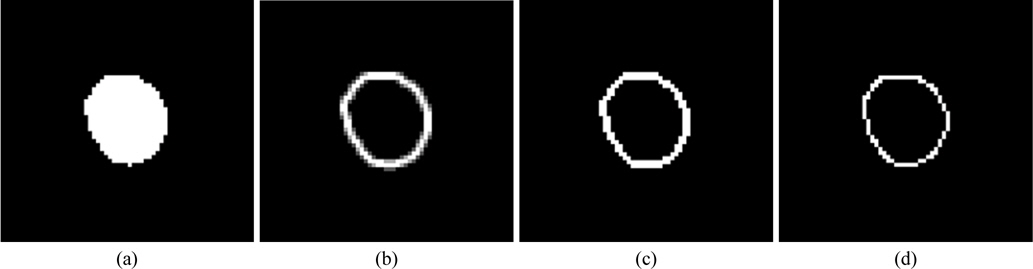
The cross section method uses the 3D surface data, the cross section being extracted at a certain height from the bottom of the hole, as shown in Fig. 1(a). Generally, an arbitrary height at 5 to 10% of hole depth is used for such bottom CD measurement; in this paper we choose 5%. The diameter is calculated by fitting the boundary data points of the cross section to a circle. To obtain the boundary data points, a Sobel edge-detection algorithm is used [13]. The result of edge detection is depicted in Fig. 1(b). The final boundary data points consisting of a one-pixel line are acquired by binarization (thresholding) and thinning of the edge image, as shown in Figs. 1(c) and 1(d). By leastsquares circle fitting, the diameter of the TSV is determined.
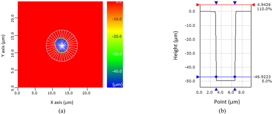
The profile analysis method also uses 3D surface data, where a profile is extracted from the data at every degree around the center of the hole, as shown in Fig. 2(a). For each profile, two points crossing the same height from the bottom of the hole are gathered. These two points are the intersections between the profile of the TSV (black solid line) and the blue horizontal line shown in Fig. 2(b). The fractional height of 5%, the same as in the cross section method, is used for the measurement. The diameter is calculated by least-squares circle fitting to these data points.
2.3. Tomographic Image Analysis Method
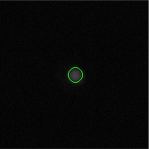
The tomographic image analysis method uses a tomographic image created from the bottom of the hole. This tomographic image is reconstructed from the focused image data for each pixel of the images captured by the camera's CCD through a 3D objective lens during vertical scanning of the 3D measurement using white-light scanning interferometry. Edge points at the bottom of the hole are detected in the tomographic image by a subpixel edge-detection algorithm [14], and the diameter is calculated by least-squares circle fitting of these edge data points, as shown in Fig. 3, where the green line indicates the fitted circle.
2.4. Two-Dimensional Gaussian Fitting Method
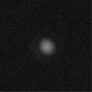
For the bottom of the hole of the TSV, due to the high aspect ratio, light attenuation near the edge still occurs, even though the measurement is performed using low numerical aperture interferometry. Depending on the fluctuations in attenuation, the relative repeatability of the bottom CD measurement using the 3D surface data may deteriorate. It also makes the edge blurry in the tomographic image, as shown in Fig. 4. Consequently, the relative repeatability of the bottom CD measurement using the tomographic images gets worse. To improve repeatability, a two-dimensional Gaussian fitting method is proposed as a postprocessing method. A two-dimensional Gaussian fitting model is applied to the converted 3D surface data for the tomographic image of the bottom of the TSV, and the bottom CD can be evaluated.
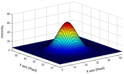
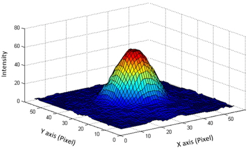
The tomographic image of the bottom of the hole is converted to 3D surface data, where the intensity of each pixel is displayed as the height, as shown in Fig. 5. This converted 3D surface shape is similar to a two-dimensional Gaussian curve, so a two-dimensional Gaussian fitting is chosen for the modeling. Figure 6 shows the result of the two-dimensional Gaussian fitting of the converted 3D surface data.
The equation for the two-dimensional Gaussian fitting model is shown in Eq. (1)
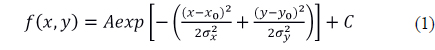
where
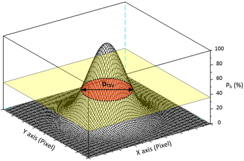
Assuming the cross-sectional shape of the hole of the TSV is a circle (

From Eq. (2),
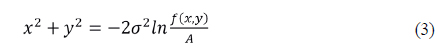
The ratio of
Thus Eq. (3) can be rewritten as

From Eq. (4), the radius of the circle can be calculated, and therefore

In Eq. (5)
III. EXPERIMENTS AND DISCUSSION
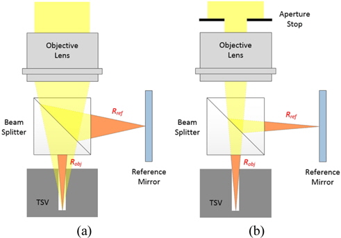
The low numerical aperture white-light scanning interferometry described by Jo et al. [10] is used for the experiment. A TSV hole with high aspect ratio makes it difficult for light to reach the bottom. The intensity of the interference signal from the white-light interferometry, denoted by

For the measurement of a high-aspect-ratio hole, the aperture is positioned ahead of the objective lens for implementing low numerical aperture interferometry, as shown in Fig. 8(b). This additional aperture limits the maximum angle of the light incident upon the object, thus making it possible for light to reach the bottom of the hole. As a result, the intensity of the interference signal at the bottom of the TSV is improved remarkably.
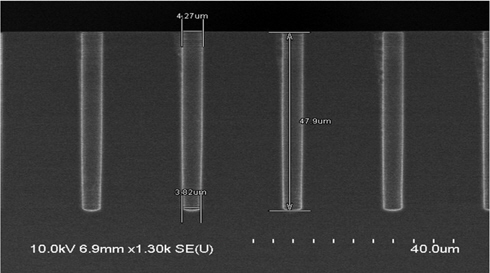
To evaluate the performance of the proposed methods for bottom CD measurements, a TSV sample with a high aspect ratio of 11.2 is precisely measured with SEM as a reference. Figure 9 shows the SEM measurement results for the sample. The diameter of the hole is 4.27 μm, the depth is 47.9 μm, and the diameter at the bottom of the hole is 3.82 μm. Next the TSV sample is measured 20 times repeatedly for evaluation, and the concept of the relative repeatability of the TSV measurement is defined as

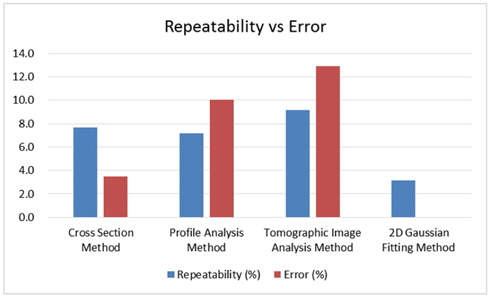
The cross section method was applied to the TSV sample, where the average diameter was measured as 3.954 μm, with 3 standard deviations being 0.303 μm and a relative repeatability of 7.7%. The profile analysis method yielded an average diameter of 4.205 μm with 3 standard deviations being 0.303 μm, for a relative repeatability of 7.2%. The tomographic image analysis method gave an average diameter of 3.328 μm with 3 standard deviations being 0.305 μm, for a relative repeatability of 9.2%.
For the two-dimensional Gaussian fitting method, the bottom CD value of the TSV sample measured with SEM, 3.82 μm, is used for the reference diameter to set
A comparison of these results is shown in Table 1 and Fig. 10. The errors of the cross section method, profile analysis method, and tomographic image analysis method are 3.5%, 10.1% and −12.9% respectively. The two-dimensional Gaussian fitting method is excluded from this comparison in terms of accuracy, because the bottom CD value of the SEM measurement result was used as the reference to calculate the diameter of the hole of the TSV. The average diameter of the cross section method is closest to the reference value, while the relative repeatability is best for the two-dimensional Gaussian fitting method.
[TABLE 1.] Comparison of the results of TSV bottom CD measurements
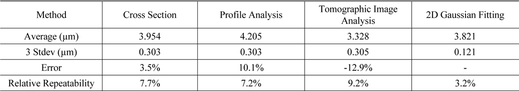
Comparison of the results of TSV bottom CD measurements
For both accuracy and relative repeatability, the tomographic image analysis method performs worst. Because of the light attenuation near the edge of the bottom of the TSV, the tomographic image is blurred severely and the measured diameter becomes much smaller than the reference. The positions of the detected edge data points fluctuate greatly, depending on the strength of the blurring, which leads to poor relative repeatability.
Comparing the cross section method to the profile analysis method, even though they use the same 3D surface data the average diameter of the cross section method is 0.251 μm smaller than that of the profile analysis method. Due to its pixel operations (edge detection and thinning), the result of the cross section method is 1-2 pixels smaller than the actual size of the measured 3D surface data. The pixel resolution is 0.18 μm/pixel at the magnification of 20x used in this experiment, so a difference of 0.251 μm, which is the same as about 1.4 pixels, is introduced. Here the actual size of the measured 3D surface data can be represented by the result of the profile analysis method, because there is no preprocessing to obtain the sampling data points. Thus the difference of 0.251 μm can occur between two methods.
The relative repeatability of the profile analysis method is a little higher than that of the cross section method. Actually, the profile analysis method is also proposed to improve the relative repeatability of the CD measurement using the 3D surface data by increasing the number of sampling data points. From the profile extraction scheme of the profile analysis method, 360 sampling data points are obtained. This number is about six times more than that of the cross section method, but the improvement of the relative repeatability is very small.
Among all these methods, the two-dimensional Gaussian fitting method provides the best relative repeatability. The improvement is about a factor of three compared to the tomographic image analysis method, which uses the same tomographic image. However, an additional measurement has to be conducted to get the reference diameter for determining
TSVs are essential for electrically connecting vertically stacked wafers in the 3D semiconductor packaging process. Thus it is very important to verify that the depths and diameters of the TSVs are created as designed. In this paper, we propose and demonstrate three kinds of direct measurement methods and one postprocessing method for examining the bottom CD of TSVs using white-light scanning interferometry. The experiments are conducted with a realistic TSV sample having a high aspect ratio of 11.2, and the performance of the proposed methods is verified by comparison to SEM measurement results. Among the three kinds of direct measurement methods, the cross section method gives the most accurate CD data with an error of only 3.5%. The diameter of the TSV can be easily evaluated by the direct measurement method, but the relative repeatability is not good enough to apply the method to fabrication monitoring. To improve the relative repeatability of the bottom CD measurement, the two-dimensional Gaussian fitting method using a modeling technique is proposed as a postprocessing method, and with it we have achieved a relative repeatability of 3.2%. It is expected that the proposed CD measurement methods will be used as monitoring tools for development of the 3D semiconductor packaging process, as well as in other areas that require CD measurement using 3D measurement data.