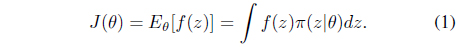
Many recent theoretical developments in the field of machine learning and control have rapidly expanded its relevance to a wide variety of applications. In particular, a variety of portfolio optimization problems have recently been considered as a promising application domain for machine learning and control methods. In highly uncertain and stochastic environments, portfolio optimization can be formulated as optimal decision-making problems, and for these types of problems, approaches based on probabilistic machine learning and control methods are particularly pertinent. In this paper, we consider probabilistic machine learning and control based solutions to a couple of portfolio optimization problems. Simulation results show that these solutions work well when applied to real financial market data.
Recent theoretical progress in the field of machine learning and control has many implications for related academic and professional fields. The field of financial engineering is one particular area that has benefited greatly from these advancements. Portfolio optimization problems [1–8] and the pricing/hedging of derivatives [9] can be performed more effectively using recently developed machine learning and control methods. In particular, since portfolio optimization problems are essentially optimal decision-making problems that rely on actual data observed in a stochastic environment, theoretical and practical solutions can be formulated in light of recent advancements. These problems include the traditional mean-variance efficient portfolio problem [10], index tracking portfolio formulation [6–8, 11], risk-adjusted expected return maximizing strategy [1, 2, 12], trend following strategy [13–17], long-short trading strategy (including the pairs trading strategy) [13, 18–20], and behavioral portfolio management.
Modern machine learning and control methods can effectively handle almost all of the portfolio optimization problems just listed. In this paper, we consider a solution to the trend following trading problem based on the natural evolution strategy (NES) [21–23, 25] and a risk-adjusted expected profit maximization problem based on an approximate value function (AVF) method [27–30].
This paper is organized as follows: In Section 2, we briefly discuss relevant probabilistic machine learning and control methods. The exponential NES and iterated approximate value function method, which are the two main tools employed in this paper, are also summarized. Solutions to the trend following trading problem and the risk-adjusted expected profit maximization problem as well as simulation results using real financial market data are presented in Section 3. Finally, in Section 4, we present our concluding remarks.
2. Modern Probabilistic Machine Learning and Control Methods
In this section, we describe relevant advanced versions of the NES and AVF methods that will be applied later in this paper.
The NES method belongs to a family of evolution strategy (ES) type optimization methods. Evolution strategy, in general, attempts to optimize utility functions that cannot be modeled directly, but can be efficiently sampled by users. A probability distribution (typically, a multi-variate Gaussian distribution) is utilized by NES to generate a group of candidate solutions. In the process of updating distribution parameters based on the utility values of candidates, NES employs the so-called natural gradient [23, 31] to obtain a sample-based search direction. In other words, the main idea of NES is to follow a sampled natural gradient of expected utility to update the search distribution. The samples of NES are generated according to the search distribution π(·∣
Note that by the log-likelihood strategy, the gradient of the expected utility with respect to the search distribution parameter

Hence, when we have independent and identically distributed samples,

It is widely accepted that using the natural gradient is more advantageous than the vanilla gradient when it is necessary to search optimal distribution parameters while staying close to the present search distribution [23, 31]. In the natural gradient based search method, the search direction is obtained by replacing the gradient ∇
1. For i = 1, · · · , n Draw a sample zi from the current search distribution. Compute the utility of the sample, f(zi). Compute the gradient of the log-likelihood, ∇θ logπ(zi|θ). end
2. Obtain the Monte-Carlo estimate of the gradient:

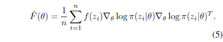
3. Obtain the Monte-Carlo estimate of the Fisher information matrix:
4. Update parameter θ of the search distribution:

The procedure shown above is a basic form of NES and can be modified based on the application. For example, the concept of the baseline can be employed to reduce the estimation variance [21]. Recent improvements to the NES procedure can be found in [21–23, 25], and one of the most remarkable improvements is the exponential NES [23, 25]. The main idea of the exponential NES method is to represent the covariance matrix of the multivariate Gaussian distribution,
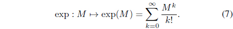
Two remarkable advantages of using the matrix exponential are that it enables the covariance matrix to be updated in a vector space, and it makes the resultant algorithm invariant under linear transformations. The key idea of the exponential NES is the use of natural coordinates defined according to the following change of variables [23]:

where
Another tool used in portfolio optimization applications of this paper is a special class of approximate value function methods [27–30]. In general, stochastic optimal control problems can be solved by utilizing state value functions, which estimate performance at a given state. The solutions of stochastic optimal control problems based on the value function are called dynamic programming. For more details on the various applications of dynamic programming, please refer to [32, 33]. Solving stochastic control problems by dynamic programming corresponds to finding the best state-feedback control policy

to optimize the performance index of specified constraints and dynamics

where
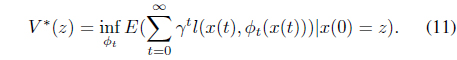
Note that the optimal performance index value is

In operator equation form, this fixed point property can be written as

where

Because it is hard to compute optimal control policy that satisfies the Bellman equation except special case [32], the AVF, :

with , it is ensured that is a lower bound of the optimal state value function V* [27, 29]. Also by optimizing this lower bound via convex optimization, the iterated AVF approach finds the approximate state value functions, , and the associated policies Note that in this step, the associated iterated AVF policies are obtained by

for

for
3. Machine Learning and Control Based Portfolio Optimization
In this section, we present probabilistic machine learning and control based solutions to two important portfolio optimization problems: the trend following trading problem and the riskadjusted expected profit maximization problem. The first topic of our portfolio application concerns trading strategy. There have been a great deal of theoretical studies on trading strategies in financial markets; however, a majority of them are focused on the contra-trend strategy, which includes trading policies for a mean-reverting market [14]. Research interests in trendfollowing trading rules are also growing. A strong mathematical foundation has led to some important theorems regarding the trend following trading strategy [14–17]. We consider an exponential NES based solution to find an efficient trend following strategy. One of the key references for our solution is the stochastic control approach of Dai et al. [14, 15]. In [14], the authors considered a bull-bear switching market, where the drift of the asset price switches back and forth between two values representing the bull market mode and the bear market mode. These switching patterns follow an unobservable Markov chain. More precisely, the governing equation for the asset price,

where

Note that in this Markov chain generator, λ1 and λ2 are the switching intensities for the bull-to-bear transition and bear-to- bull transition, respectively. In [14], it is assumed that the switching market mode, {
if initially flat, and
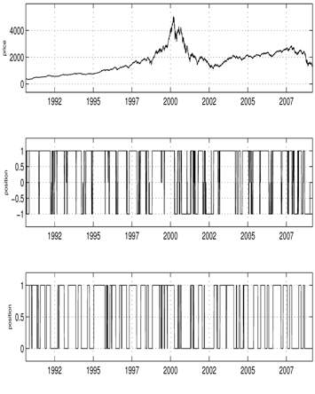
if initially long [14]. The results of [14] are mathematically rigorous and establish a strong theoretical justification for the trend following trading theory. We utilize a less mathematical, but hopefully easier to understand approach, which is based on the exponential NES method [23, 25] for the trend following trading problem. Note that in the exponential NES approach, the performance index may be chosen with more flexibility. This paper extends our previous work on this topic [13] in two ways. First, we utilize a more advanced version of the NES–the exponential NES [23, 25]–that is now the state-of-the-art method in the field. Second, we focus on more flexible long-flat-short type trading rules whereas our previous paper considered only the long-flat strategy. According to [14], there exist two monotonically increasing optimal sell and buy boundaries, and , in case of the finite-horizon problem for obtaining the optimal trend following long-flat type trading rule. When long-term investments are emphasized, the behavior of the system is similar to the infinite horizon case, and these threshold functions can be approximated by constants [14, 15]. Following this approximation scheme, we try to find threshold constants for all possible transitions that can occur in long-flat-short type trading, i.e., by applying the exponential NES method [23, 25]. The price-series sample paths generated in accordance with the switching geometric Brownian motion (18) are required during the training phase. Simulating both Markov chains and geometric Brownian motions is not difficult; thus, the price-series sample path generation can be performed efficiently. By combining the thresholds found by the exponential NES method together with the Wonham filter [14, 34] to estimate the conditional probability that the mode of the market is bull, one can obtain a long-flat-short type trend following trading strategy. To illustrate the applicability of the exponential NES based trading strategy, we considered the problem of determining a trend following trading rule for the NASDAQ index. For the example, NASDAQ closing data from 1991 to 2008 was considered (see Fig. 2). According to the estimation results of [14], the parameters of the switching geometric Brownian motion for the NASDAQ are as follows: μ1 = 0:875, μ2 = −1.028, σ1 = 0.273, σ2 = 0.35, σ = 0.31, λ1 = 2.158, λ2 = 2.3, where
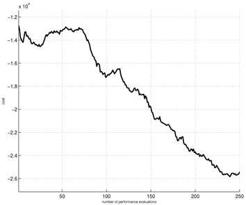
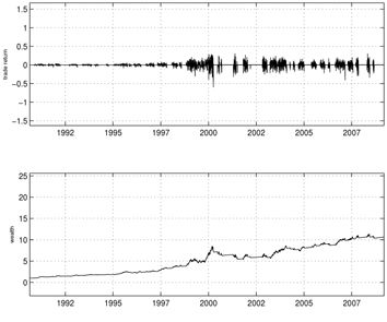
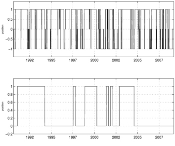
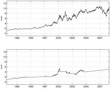
Figures 1-6 show the simulation results for the exponential NES based trend following trading rules. For these simulations, we set the initial wealth to one. Figure 1 shows the learning curve, which graphs the average total cost sums versus the policy update over a set of 10 simulation runs. As shown in the curve, the exponential NES method exhibits desirable behavior within less than 250 policy updates. This indicates that the exponential NES method works well for finding a long-flat-short type trading strategy. Figure 2 shows the NASDAQ index values together with the long-flat-short trading signals resulting from a policy obtained by the exponential NES method over the entire period. For comparison purposes, we also show the long-flat trading signals obtained by the NES approach [13]. According to Fig. 2, the total number of position changes in the long-flat-short type trading strategy (2nd panel) is 345. Note that this value differs from the corresponding number of position changes in the long-flat type trading strategy (3rd panel, 100 changes) obtained by the NES approach [13]. Simulation results in Fig. 3 show that with the exponential NES based long-flat-short type trading strategy, trade returns are generally large and wealth steadily increases until it reaches 21.52 at the final time. In comparison, Fig. 4 shows that with the long-flat type trading rule, the trade returns are generally small, and wealth increases at a relatively slower rate. Its wealth value at the final time is only 10.65. From these simulation results, one can see that when
For the second application example, we considered the riskadjusted, expected profit maximization problem and utilized an AVF [27–30] based procedure to find an efficient solution. To express the risk-adjusted, expected profit maximization problem in state-space format, it is necessary to define the state and control input together with the performance index that is used as an optimization criterion. To do this, we follow the research of Boyd et al. [1, 28, 30]. We define the state vector as the collection of the portfolio positions. Let

The control input considered for this problem is a vector of trades,

executed for portfolio

where

where the total gross cash entered in the portfolio is 1

which means that only a limited amount of trading is allowed for each asset. Thus, the risk-adjusted profit maximization problem can be expressed as
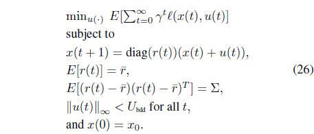
To solve this optimization problem, we utilized the iterated AVF approach [29], which is one of the most advanced AVF methods. In the iterated AVF approach, convex quadratic functions

are used to approximate the state value function at time

with The Bellman inequalities guarantee that is a lower bound of the optimal state value function [27–29]. The iterated AVF method maximizes this lower bound using convex optimization [29]. Another constraint is kuk1 ∥

where
For the Bellman inequalities in (28), we considered
The control input considered for this problem is a vector of trades,
executed for portfolio
where
which means that only a limited amount of trading is allowed for each asset. Thus, the risk-adjusted profit maximization problem can be expressed as
To solve this optimization problem, we utilized the iterated AVF approach [29], which is one of the most advanced AVF methods. In the iterated AVF approach, convex quadratic functions
are used to approximate the state value function at time
with The Bellman inequalities guarantee that is a lower bound of the optimal state value function [27–29]. The iterated AVF method maximizes this lower bound using convex optimization [29]. Another constraint is ∥
where
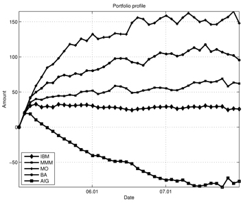
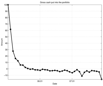
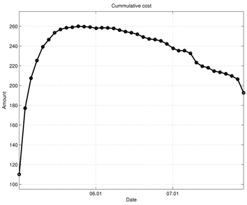
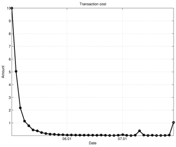
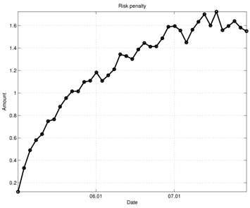
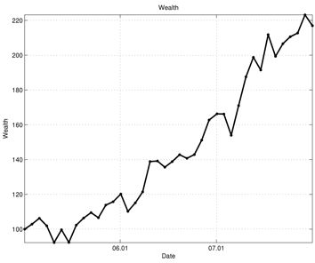
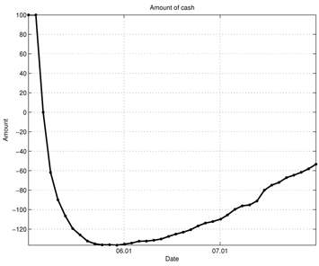
Figures 7-13 show the simulation results of the portfolio optimization example under the iterated AVF method. Figure 7 depicts the portfolio profile during the test period. From this figure, one can see that with the passage of time, the portfolio profile slowly changes its direction to increase the performance index. Figure 8 shows the gross cash put into the portfolio, and Fig. 9 plots the cumulative cost sums. From Fig. 8, it is clear cash is entered into the portfolio during the early stage of trade; as time progresses, the portfolio gains income. Furthermore, based on the trend of this figure, we can expect more profit to be derived in the later stage of trading. Figure 10 shows the transaction cost. When the portfolio is being built, the transaction cost is very high; however, it stabilizes over time. Figure 11 shows the risk penalty, which is always non-negative and increasing. Wealth history and amount of cash holdings are plotted in Figs. 12 and 13, respectively. Note that in this scenario, wealth steadily increases as trading proceeds and reaches approximately 220 (yielding a 120% profit at the end of 2007). Also note that according to Fig. 13, the amount of cash holding briefly remains at the initial value, rapidly decreases, and then slowly begins to restore itself. This behavior suggests that in the iterated AVF based trading strategy, a large amount of profit is obtained when aggressive initial investments are made with cashing out subsequently.
Machine learning and control methods have been applied to a variety of portfolio optimization problems. In particular, we considered two important classes of portfolio optimization problems: the trend following trading problem and the risk-adjusted profit maximization problem. The exponential NES and iterated approximate value function methods were applied to solve these problems. Simulation results showed that these probabilistic machine learning and control based solutions worked well when applied to real financial market data. In the future, we plan to consider more extensive simulation studies, which will further identify the strengths and weaknesses of probabilistic machine learning and control based methods, and applications of our methods to other types of financial decision making problems.