Image blur due to the focusing error of camera systems (defocus blur) is mainly a result of a certain problem of the geometric image formation and the finite depth of field of practical camera lens systems. The camera lens system with the focusing error tends to defocus objects and blur the acquired images. This kind of image blur caused by the focusing error or by an imperfect imaging lens system with defocusing aberration will cause serious image degradation. Many kinds of image processing techniques have been developed to restore the original image [1-3]. Most of these techniques estimate the point-spread function (PSF) associated with the image acquisition system which carries out space-invariant deconvolution based on the estimated blurring function for image restoration. In addition to the applications related to image restoration or sharpening, defocus blur is also considered as an important visual cue for image quality assessment [4, 5] and super resolution image reconstruction [6, 7]. For the images captured with small depth-of-field, defocus blur can be used for image segmentation or interested region detection [8, 9]. Moreover, depth recovery from a single camera can be achieved by measuring the blur extent of the captured defocused image [10, 11]. In the above applications, the identification of defocus blur parameters plays a central role in their underlying techniques. Moreover, these kinds of techniques are able to identify the blur parameters for specific application domains. However, the estimation of a blur does not necessarily give the true parameter estimate [12]. As a result, the analysis is simply carried out based on the comparison between the defocused blur image and original image.
In this paper, we adopted the Joint transform correlator (JTC) to carry out the comparison between the defocused blur image and original image. JTC has shown remarkable achievements and is a useful alternative to the other optical systems [13-15] for pattern recognition and target tracking applications. The typical advantage of the JTC is that it uses a type of real time optical system which quantitatively compares images by measuring correlation peaks [16]. Recently, the JTC shows a unique application in the color comparison and color difference measurement [17]. This works presented the close relation between the color difference and the correlation peaks by decomposing the red, green, and blue components from the original images. In this paper, we presented a simple technique to estimate qualitatively the extents of blurring and to restore the original image by using the JTC. The correlation peaks obtained by the JTC play an essential role as the blur parameters to estimate quantitatively the extents of the blurring in detail. The correlation peaks are used to calculate the focusing error which results in the restoration of original image by calibrating the defocused camera. In the following sections, the relation between the correlation and the focusing error concerning the OTF (optical transfer function) and the JTC system in detail. Section III describes simulation results and discusses a possibility of the restoration of original image and the calibration of the camera lens with the defocused aberration, and finally some comments are contained in the conclusion section.
II. BLURRING EXTENTS AND CORRELATION PEAK
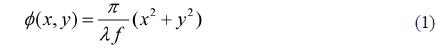
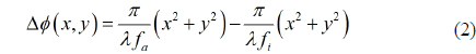
One of the easiest aberrations to deal with mathematically is a simple focusing error of the lens. When a focusing error is present, the center of curvature of the spherical wavefront converging towards the image of an object is formed either to the left or to the right of the image plane. Considering an on-axis point for simplicity, the phase distribution across the exit pupil is of the form
where
where
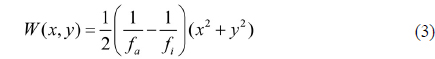
which is seen to depend on the quadratic space variables in the exit pupil. For the assumption of a square aperture of width 2
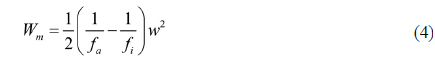
The number
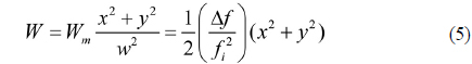
If the path-length error

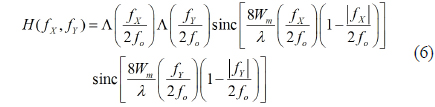
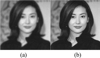
We want to know the relation between the OTF of Eq. (6) caused by the focusing error and the extents of the image blurring caused by this focusing error. Now we prepare a JTC system to investigate the effect of the focusing error on the image blurring. Figure 1 shows the optical structure of the JTC system for the investigation of the defocusing effect on the correlation peak and PSNR. The optical system of Fig. 1 is composed of two parts, the image capture camera part and the JTC part. The image capture camera part is composed of a camera lens system which captures the original image on the LCD come from a PC. The captured image will be blurred if the camera lens is defocused. The blurred image comes into the PC and is combined with the original image to form a joint input image on LCD 1. Let us call the reference image

The joint power spectrum (JPS) on the Fourier plane, which is called the intensity of this interference fringe pattern, can be expressed as
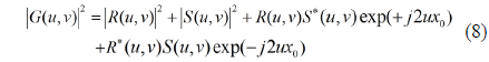
Here, * is the phase conjugate,
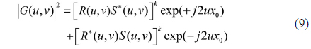
If the reference image perfectly matches the sample image and there is no phase error between the reference image and the sample image, the output can be expressed as
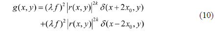
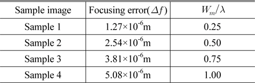
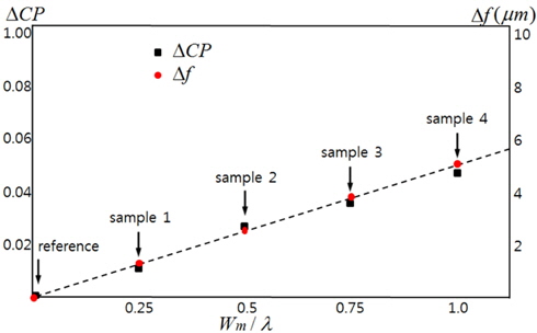
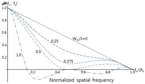
Figure 2 shows the computer simulated results of the OTF derived from Eq. (6) for various values of
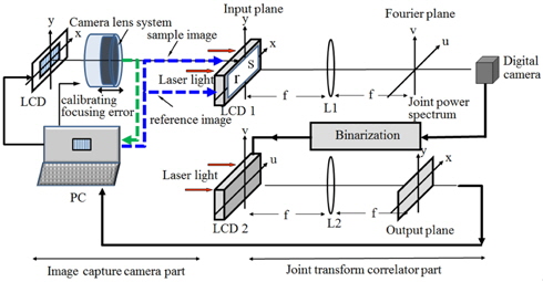
[TABLE 1.] Results of the focusing error for various values of Wm/λ

Results of the focusing error for various values of Wm/λ
[TABLE 2.] Correlation peaks of the sample images measured by the JTC system
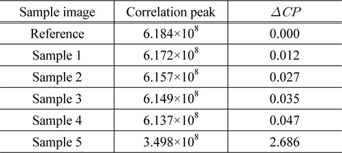
Correlation peaks of the sample images measured by the JTC system
In this paper, we presented a new technique of estimating the extents of blurring effect caused by defocusing a camera lens using the JTC. In addition, we presented a possibility of calibration of the blurred images by finding the focusing error calculated from the measured correlation peak. Thus, we can conclude that a camera lens system with the aberration of the defocusing error can be calibrated by finding