A general linearly constrained adaptive array is examined in the weight vector space to illustrate the array performance with respect to the gain factor. A narrowband linear adaptive array is implemented in a coherent signal environment. It is shown that the gain factor in the general linearly constrained adaptive array has an effect on the linear constraint gain of the conventional linearly constrained adaptive array. It is observed that a variation of the gain factor of the general linearly constrained adaptive array results in a variation of the distance between the constraint plane and the origin in the translated weight vector space. Simulation results are shown to demonstrate the effect of the gain factor on the nulling performance.
If the desired signal is uncorrelated with incoming interference signals, a linearly constrained adaptive array successfully estimates the desired signal by reducing the interference signals [1]. If the desired signal is correlated partially or totally (i.e., coherent) with the interference signals, the desired signal is partially or totally cancelled in the array output depending on the extent of correlation between the desired signal and the interference signals.
Some methods, such as the spatial smoothing approach [2, 3], master-slave type array processing [4], alternate mainbeam nulling method [5], and general linearly constrained adaptive array [6], have been proposed to prevent the signal cancellation phenomenon in a correlated signal environment. A drawback of the methods proposed in [2-5] is that they employ additional hardware or algorithms to reduce the effect of the coherent interferences.
In this study, the general linearly constrained adaptive array is examined in the weight vector space to find the nulling performance in [6] in terms of the gain factor, which turns out to be the reduction of the gain in the look direction in the translated weight vector space. It is shown that the variation of the gain factor results in the variation of the distance between the constraint plane and the origin in the translated weight vector space, which has a geometric effect of shifting the constraint plane with respect to the origin.
The simulation results are shown to illustrate the nulling performance with respect to the gain factor. It is shown that the general linearly constrained adaptive array performs better than the linearly constrained adaptive array with respect to the elimination of the coherent interferences.
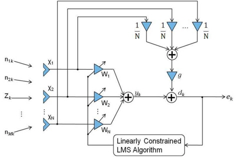
It is assumed that a desired signal is incident from a known direction (i.e., the look direction) while coherent interferences come from unknown directions on the narrowband general linearly constrained adaptive array with
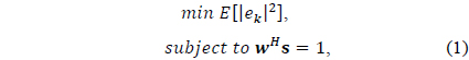
To find the array weights that optimally estimate the desired signal in the look direction while eliminating the undesired interference signals as much as possible, we solve the following optimization problem in which the mean square error is minimized subject to the unit gain constraint in the look direction.

where the error signal between the adaptive array output and the desired response is given by

the output of the adaptive array is represented as

the desired response is given by

and the signal vector, the weight vector


where
It can be shown that the mean squared error

where

The method of Lagrange multipliers [1] is used for finding the optimal solution by solving the unconstrained optimization problem with the objective function

where λ denotes a Lagrange multiplier.
Here, the optimum weight vector is given by

It is observed in (11) that the optimum weight vector lies between the uniform weight of the conventional beamformer and the optimum weight vector for the unit gain constraint depending on the value of the gain factor.
III. OPTIMUM WEIGHT VECTOR IN THE TRANSLATED WEIGHT VECTOR SPACE
We designate the weight vector
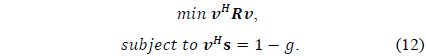
Solving (12) by using the Lagrange multiplier method, we obtain the optimum weight vector as

The optimum weight vector in (13) is for the unit gain constraint scaled by (1 –
IV. GENERAL LINEARLY CONSTRAINED LMS ALGORITHM
The steepest descent method [7] is employed to find the iterative solution for the optimum weight vector, where the next weight vector is given by the current one added by the negative gradient with respect to

where
The objective function is given by

Applying the constraints in (12) to (14) to find the value of

where


where ∗ denotes a complex conjugate.
Eq. (18) is called the general linearly constrained least mean square (LMS) algorithm. In (19), it is observed that the updated weight vector
Thus, a variation of the gain factor results in a variation of the distance between the constraint plane and the origin in the translated weight vector space (i.e., an increase in the gain factor results in a decrease in the distance). This phenomenon has an effect on the nulling performance of the general linearly constrained adaptive array in terms of the gain factor.
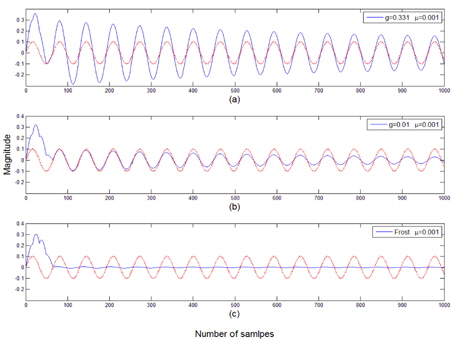
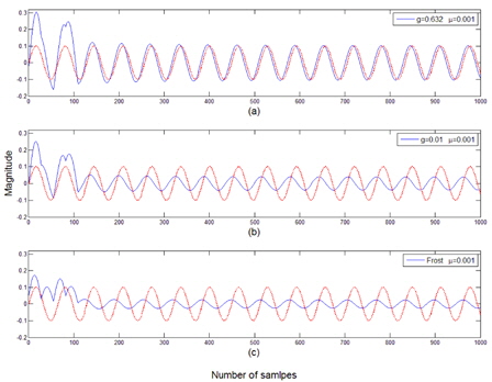
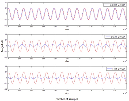
To illustrate the nulling performance of the general linearly constrained adaptive array in terms of the gain factor, the simulation results in [6] are redisplayed for the cases of one and two coherent interferences.
A narrowband linear array with 7 equispaced sensor elements is employed to examine the performance of the general linearly constrained adaptive array. The incoming signals are assumed to be plane waves. The desired signal is assumed to be a sinusoid incident on the linear array at the array normal. The cases for one and two coherent interferences are simulated. The nulling performances are compared with respect to the gain factor
>
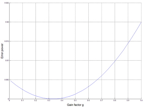
A. Case of One Coherent Interference Case
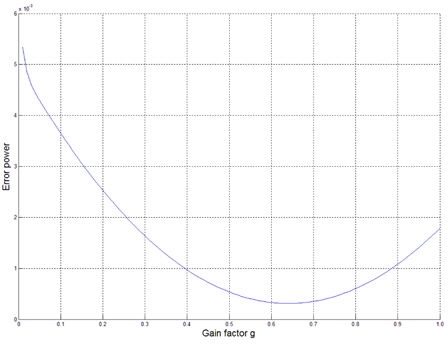
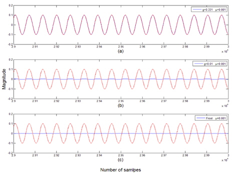
It is assumed that a coherent interference is incident at 30° from the array normal. The variation of the error power between the array output and the desired signal is displayed in terms of the gain factor
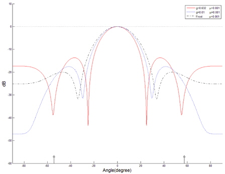
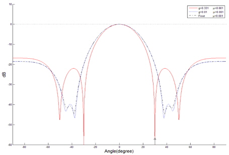
The beam patterns are shown in Fig. 5, in which the case for
>
B. Case of Two Coherent Interferences
It is assumed that two coherent interferences are incident at -54.3° and 57.5° from the array normal. The variation of the error power between the array output and the desired signal is displayed in Fig. 6. The optimum value of
A narrowband general linearly constrained adaptive array is examined in the weight vector space to calculate the array performance with respect to the gain factor in a coherent signal environment. It is observed that a variation of the gain factor results in a variation of the distance between the constraint plane and the origin in the translated weight vector space. This phenomenon has an effect on the nulling performance of the general linearly constrained adaptive array. Further, it is shown that the general linearly constrained adaptive array performs better than the linearly constrained adaptive array.